Fitting GEV to Block Maxima Data

Introduction

In our previous lesson, we learned how to select the most appropriate statistical model for a dataset by balancing goodness-of-fit with model complexity, using tools like AIC, BIC, and the Likelihood Ratio Test. These methods work well for modeling the main body of a loss distribution. However, in risk management, our primary concern often isn't the typical, everyday claim. It's the rare, catastrophic event lurking in the tail of the distribution—the "black swan" that can threaten an entire company's solvency.

Standard distributions that fit the bulk of the data often provide a dangerously poor fit to these extreme tails. This is where Extreme Value Theory (EVT) becomes an indispensable part of the actuary's toolkit. Today, we'll delve into the first of two primary EVT approaches. We will explore how the maxima of data samples behave and how we can model them using the Block Maxima Method and the Generalized Extreme Value (GEV) distribution.

The Theory of Extremes: An Analogue to the Central Limit Theorem

Your background in probability theory makes you intimately familiar with the Central Limit Theorem (CLT). The CLT is a cornerstone of statistics, telling us that the distribution of the sum (or average) of many independent and identically distributed (i.i.d.) random variables, when properly normalized, converges to a Gaussian distribution, irrespective of the underlying distribution of the variables themselves.

EVT begins with a wonderfully analogous question: What about the maximum? Is there a similar limiting distribution for the maximum of a sample? The answer is yes, and it is provided by the Fisher-Tippett-Gnedenko theorem.

The following video provides an excellent introduction to this concept, drawing a direct parallel between the CLT for sums and the foundational theorem of EVT for maxima.

Extreme value theory (QRM Chapter 5)

This video, from the "QRM Tutorial" series, offers a clear and mathematically sound introduction to Extreme Value Theory.

Please watch the section from the start of the main introduction. The lecturer masterfully frames EVT by placing models for sums (governed by the CLT) in his "right pocket" and introducing the need for new models for maxima, which he'll place in his "left pocket." This analogy powerfully establishes the motivation for a separate theory of extremes.

As the video explains, just as the Gaussian distribution is the universal model for sums, a different family of distributions forms the universe of models for maxima. This family is known as the Generalized Extreme Value (GEV) distribution.

The Generalized Extreme Value (GEV) Distribution

The Fisher-Tippett-Gnedenko theorem states that the only possible non-degenerate limit for the distribution of the normalized maximum of an i.i.d. sample is the GEV distribution. This powerful result means that regardless of whether your original data is Normal, Exponential, or Pareto, the distribution of its block maxima will tend toward a GEV.

The GEV distribution is defined by three parameters:

Location parameter, $μ$ : Shifts the distribution along the x-axis.
Scale parameter, $θ > 0$ : Stretches or compresses the distribution.
Shape parameter, $ξ$ : This is the most important parameter. It governs the tail behavior of the distribution and determines its fundamental character.

The cumulative distribution function (CDF) for the GEV is given by:

H_{ξ, μ, θ} (x) = {exp (- [1 + ξ (\frac{x - μ}{θ})]^{- 1/ ξ}) exp (- e^{- (x - μ) / θ}) for ξ \neq = 0 for ξ = 0

The value of the shape parameter, $ξ$ , classifies the distribution into one of three types.

[PDF] ASTAM-22-23: Chapter 5 of Quantitative Enterprise Risk ... - SOA.org

This excerpt from "Quantitative Enterprise Risk Management" provides the formal definitions we need.

First, read the section that introduces the three primary types of extreme value distributions: the three distributions. Then, see how they are unified into a single GEV distribution in the paragraphs beginning the GEV definition. Finally, read the statement of the Fisher–Tippett–Gnedenko Theorem.

The three types of GEV distribution, determined by the shape parameter $ξ$ , are:

Type I: Gumbel ( $ξ = 0$ ): This corresponds to underlying distributions with "light" tails that decay exponentially, such as the Normal, Exponential, and Lognormal distributions.
Type II: Fréchet ( $ξ > 0$ ): This is the most important type for financial and insurance applications. It arises from "heavy-tailed" underlying distributions like the Pareto, Cauchy, and log-gamma. These distributions have tails that decay as a power law, allowing for more extreme events than the Gumbel.
Type III: Weibull ( $ξ < 0$ ): This type corresponds to distributions with a finite upper bound, like the Uniform or Beta distributions. It is less common in financial risk modeling but appears in other fields, such as modeling rainfall or human lifespan.

The following resource provides a useful table that maps common underlying distributions to their corresponding GEV family.

[PDF] Extreme value theory - Actuarial Education

This study note from ActEd provides a practical summary of the GEV distribution.

Focus on the table under section 3.3 Underlying distributions, which starts with the full table. This table is an excellent reference for understanding which type of tail behavior to expect from different models.

The Block Maxima Method

The theory is elegant, but how do we apply it to a real dataset? The most direct application of the Fisher-Tippett-Gnedenko theorem is the Block Maxima (BM) method.

The procedure is simple and intuitive:

Take your time-series data (e.g., daily insurance losses) and divide it into non-overlapping blocks of equal size. A common choice is to use one year as the block size.
For each block, identify the single largest observation.
The collection of these maxima—one from each block—forms a new dataset. These are your "block maxima."
According to the theory, this new dataset of block maxima can be treated as an i.i.d. sample from a GEV distribution.
Finally, you can fit the GEV distribution to this sample of block maxima using standard statistical techniques, most commonly Maximum Likelihood Estimation (MLE), to find the parameters $μ, θ$ , and $ξ$ .

This chart illustrates the Block Maxima method. The original data points (black dots) are partitioned into four blocks. From each block, the maximum value (M1, M2, M3, M4) is extracted. These four maxima then form the new dataset to which the GEV distribution is fitted.

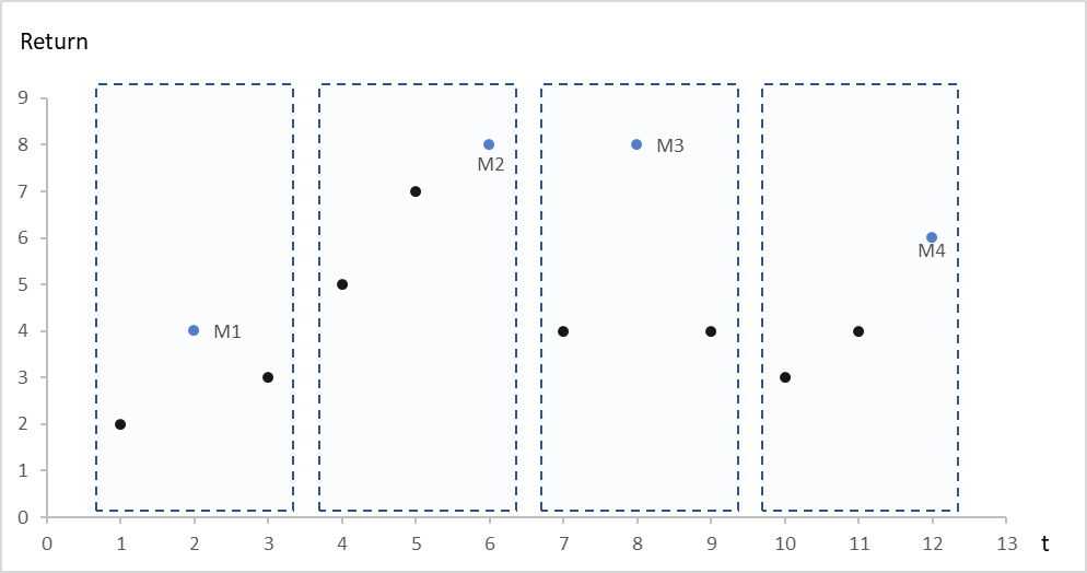
The primary challenge in the Block Maxima method is choosing the block size. This choice involves a classic statistical trade-off between bias and variance.

Extreme value theory (QRM Chapter 5)

Let's return to the QRM Tutorial video for a practical discussion of this method.

Watch the segment from the explanation of the Block Maxima method. Pay close attention to the discussion of the bias-variance trade-off: Large blocks (e.g., 5-year periods) lead to maxima that better satisfy the asymptotic theory (low bias), but you end up with very few data points, leading to high variance in your parameter estimates. Small blocks (e.g., monthly) give you many data points for estimation (low variance), but the maximum of a small sample may not be "extreme" enough for the limiting distribution to be a good approximation (high bias).

There is no universally optimal block size; it often depends on the data's characteristics and natural cycles (e.g., annual seasonality).

A Practical Example: Fitting GEV to Stock Market Losses

Let's walk through a complete example of applying the Block Maxima method to real financial data. We will use a dataset of monthly losses on the S&P/TSX stock index.

[PDF] ASTAM-22-23: Chapter 5 of Quantitative Enterprise Risk ... - SOA.org

This final section of the "Quantitative Enterprise Risk Management" reading contains a detailed worked example.

First, read the section "5.3.4 Estimating the GEV Parameters" to understand how Maximum Likelihood Estimation is set up for the GEV. Skim the log-likelihood formula to appreciate its structure, but focus on the qualitative discussion around the data requirements trade-off. Next, carefully study Example 5.4 and Table 5.1. This is the core of our practical application. Part (a): The data is blocked annually (block size of 12 months). The GEV parameters are estimated from the 56 annual maxima. Note the parameter estimates: \hat{\mu} = 5.009, \hat{\theta} = 3.012, and most importantly, \hat{\xi} = 0.1575. Since \hat{\xi} > 0, this points to a heavy-tailed Fréchet distribution, which is exactly what we expect for financial asset returns. Part (b): The analysis is repeated with a larger block size of 24 months. Now we have only 28 block maxima. Notice that the standard errors for the parameter estimates are larger, as expected from a smaller sample size. While the point estimate for \xi has changed, it is still positive, reinforcing the conclusion of a heavy-tailed phenomenon. The value of \xi should ideally be stable across different large block sizes.

This example brilliantly demonstrates the entire process: blocking the data, extracting maxima, fitting the GEV distribution via MLE, and interpreting the results, including the practical consequences of the block size choice.

Conclusion

Today we took our first major step into the world of Extreme Value Theory. We have seen that by focusing on the maximum values within data blocks, we can leverage a powerful theoretical result—the Fisher-Tippett-Gnedenko theorem—to model extreme events in a robust and principled way, moving beyond the limitations of standard distributions.

Key Takeaways:

Standard statistical models often fail to capture tail behavior accurately, which is critical for risk management.
The Fisher-Tippett-Gnedenko theorem is the EVT equivalent of the Central Limit Theorem, stating that the normalized maxima of i.i.d. samples converge to the Generalized Extreme Value (GEV) distribution.
The GEV distribution's character is defined by its shape parameter ( $ξ$ ), which classifies the tail as Gumbel ( $ξ = 0$ , light), Fréchet ( $ξ > 0$ , heavy), or Weibull ( $ξ < 0$ , finite endpoint).
The Block Maxima method is a practical technique for applying this theory by dividing data into blocks, extracting the maxima, and fitting a GEV distribution to this new sample.
Choosing a block size involves a critical bias-variance trade-off that requires careful judgment.

Preview of the Next Lesson

A key drawback of the Block Maxima method is its inefficiency. In each block, we discard all data points except for one, the maximum. If a block contains several large values, this approach loses potentially valuable information.

In our next lesson, we will explore an alternative and often more powerful method called Peaks-Over-Threshold (POT). Instead of looking at the maximum in a block, POT involves setting a high threshold and modeling the distribution of all values that exceed it. This leads us to the second fundamental distribution in EVT: the Generalized Pareto Distribution (GPD).

Recommended resources