Introduction to Copulas and Sklar's Theorem

Introduction

Welcome to a new module focused on one of the most powerful tools in modern risk modeling: copulas. In our previous module, culminating with the study of Extreme Value Theory, we developed a sophisticated toolkit for modeling the behavior of a single risk factor, paying special attention to its tail. We learned how to answer questions like, "What is the 1-in-200 year loss for our property insurance line?"

However, risks rarely exist in a vacuum. A major hurricane doesn't just cause property losses; it can also lead to business interruption claims, an increase in auto claims from flooding, and even affect life insurance portfolios. The true risk to an enterprise lies not just in the magnitude of individual losses, but in how these losses move together.

This lesson introduces the fundamental concept of the copula, a mathematical function that allows us to model the dependence between random variables separately from their individual behaviors. We will define what a copula is and introduce Sklar's theorem, the cornerstone result that makes this entire approach possible. By the end of this lesson, you will understand how copulas provide a far more nuanced and flexible language for describing dependence than simple correlation.

The Limits of Correlation

As a statistician, you are well-acquainted with using correlation coefficients, particularly Pearson's $ρ$ , to summarize the relationship between two variables. It's a simple, intuitive measure. However, when it comes to risk management, relying solely on linear correlation can be dangerously misleading.

To understand why, let's explore a brief reading that frames the problem.

Modeling Tail Risks: A Brief Introduction to Copulas - Medium

This article from Medium provides an excellent motivation for why we need tools beyond simple correlation in risk modeling.

Please read the introductory section, "Copulas — Why Bother?". As you read, focus on these key points: Why correlation is described as a "blunt instrument." The definition and importance of "tail dependency." The real-world examples given, such as the factory fire or the 2008 financial crisis, which illustrate the failure of models that ignore tail dependence.

The central message is that correlation measures an average association across the entire distribution, but it is often blind to what happens in the extremes, or "tails." Two asset classes might have a low correlation during normal market conditions, but in a crash, they might both plummet in value, exhibiting strong tail dependence. A model based on the average correlation would fail to capture this catastrophic co-movement.

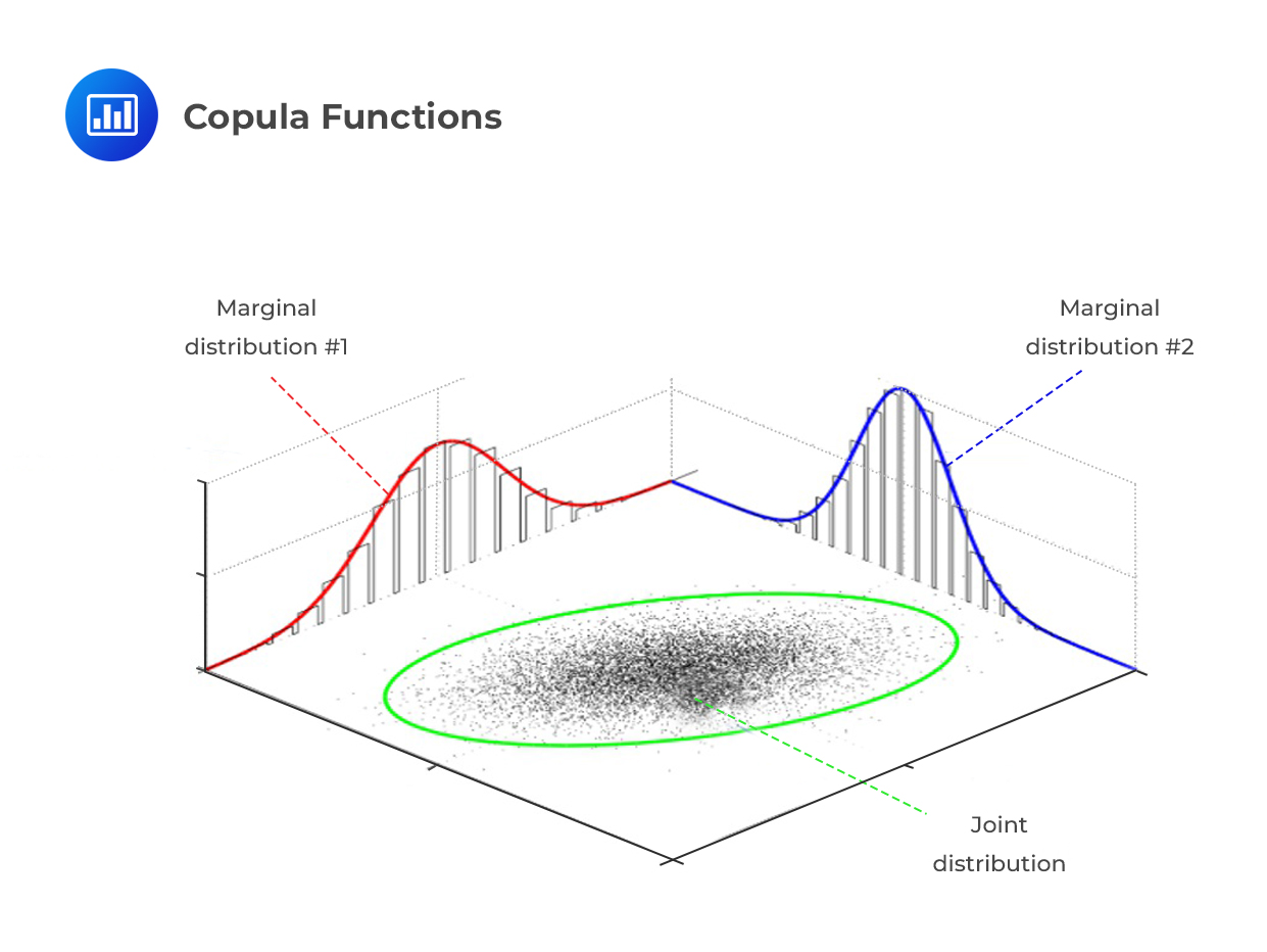
Copulas are the solution to this problem. They allow us to build a joint distribution by specifying two distinct components:

The marginal distributions for each individual risk (which we learned to model in previous modules).
A copula function, which describes the dependence structure that "couples" them together.

This image illustrates the core idea. We have two separate marginal distributions (the red and blue curves). The copula is the mechanism that joins them to create the full joint distribution (the scatter of points in the center).

Sklar's Theorem: The Foundation of Copula Modeling

The ability to separate marginals from their dependence structure is not just a convenient trick; it is formally justified by a profound result in probability theory known as Sklar's Theorem. This theorem is the bedrock of all copula modeling.

Before stating the theorem, let's watch a video that provides an intuitive introduction to the concept and the underlying mechanics.

Copulas 1: A Gentle Introduction

This video from the "Meerkat Statistics" channel offers a clear, gentle introduction to the core ideas behind copulas and Sklar's theorem.

Please watch the following two segments: Introduction (0:00 - 1:52): This will reinforce the motivation for using copulas over simple correlation. CDF Transformation and Sklar's Theorem (3:07 - 5:06): This part is crucial. It reviews the probability integral transform and then shows how Sklar's theorem applies this concept to define the copula.

The video highlights a key concept from your probability theory background: the probability integral transform. If a continuous random variable $X$ has a CDF $F_{X} (x)$ , then the transformed random variable $U = F_{X} (X)$ follows a standard uniform distribution, $U \sim Uniform [0, 1]$ .

Sklar's theorem extends this idea to the multivariate case. It states that any joint cumulative distribution function can be expressed in terms of its marginal CDFs and a copula function that links them.

Let's look at the formal statement from our course notes.

M5 Copulas | General Insurance Modelling - AM3

This resource provides the formal mathematical statement of Sklar's theorem.

Please read the section under the heading Sklar's representation theorem. Focus on the main equation presented.

As the resource shows, for a set of random variables $X_{1}, X_{2}, \dots, X_{n}$ with a joint CDF $F (x_{1}, \dots, x_{n})$ and marginal CDFs $F_{1} (x_{1}), F_{2} (x_{2}), \dots, F_{n} (x_{n})$ , Sklar's Theorem (1959) guarantees that there exists a copula function $C$ such that:

F (x_{1}, x_{2}, \dots, x_{n}) = C (F_{1} (x_{1}), F_{2} (x_{2}), \dots, F_{n} (x_{n}))

Let's break this down:

The inputs to the copula function, $u_{k} = F_{k} (x_{k})$ , are the marginal probabilities. Each $u_{k}$ is a value in $[0, 1]$ .
The copula $C$ is itself a multivariate distribution function defined on the unit hypercube $[0, 1]^{n}$ . It's the joint CDF of the uniformly distributed random variables $U_{k} = F_{k} (X_{k})$ .

If the marginal distributions are continuous, the copula $C$ is unique and can be expressed as:

C (u_{1}, \dots, u_{n}) = F (F_{1}^{- 1} (u_{1}), \dots, F_{n}^{- 1} (u_{n}))

where $F_{k}^{- 1}$ is the quantile function (the inverse CDF) of the $k$ -th marginal.

What, Exactly, is a Copula?

Sklar's theorem tells us a copula exists and connects marginals to their joint distribution. But what is the mathematical definition of a copula function itself?

Simply put, a copula is a multivariate CDF whose marginal distributions are all Uniform[0,1].

For a function $C (u_{1}, u_{2})$ to be a valid two-dimensional copula, it must satisfy a few key properties. These properties ensure that it behaves like a proper joint CDF.

M5 Copulas | General Insurance Modelling - AM3

This section of the course notes lays out the formal conditions for a function to be a valid copula, along with helpful intuitive explanations.

Focus on the section When is C a valid copula?. Pay attention to the three numbered conditions and their corresponding "heuristics".

As the reading explains, for a bivariate copula $C (u_{1}, u_{2})$ , the key properties are:

Grounding: $C (u_{1}, 0) = 0$ and $C (0, u_{2}) = 0$ . If one variable takes its minimum possible value (in the uniform space), the joint probability is zero.
Marginals: $C (u_{1}, 1) = u_{1}$ and $C (1, u_{2}) = u_{2}$ . If one variable takes its maximum possible value, the joint CDF collapses to the marginal CDF of the other. This shows the marginals are uniform.
Rectangle Inequality: For any $u_{1} \leq v_{1}$ and $u_{2} \leq v_{2}$ , we must have $C (v_{1}, v_{2}) - C (u_{1}, v_{2}) - C (v_{1}, u_{2}) + C (u_{1}, u_{2}) \geq 0$ . This ensures that the probability mass over any rectangle $[u_{1}, v_{1}] \times [u_{2}, v_{2}]$ is non-negative.

The simplest possible copula is the independence copula, given by $C (u_{1}, u_{2}, \dots, u_{n}) = u_{1} \cdot u_{2} \dots u_{n}$ . Plugging this into Sklar's theorem gives $F (x_{1}, \dots, x_{n}) = F_{1} (x_{1}) \dots F_{n} (x_{n})$ , which is exactly the definition of statistical independence. All other copulas introduce some form of dependence.

The true power of this framework, as we'll see, is its flexibility.

Copulas 1: A Gentle Introduction

Let's conclude with a clip that beautifully illustrates the "mix-and-match" flexibility that copulas provide.

Watch the final segment of the video from 10:11 to 11:05. The narrator demonstrates how different joint distributions can be created by combining various marginal distributions with different copulas.

Conclusion

In this lesson, we have laid the conceptual groundwork for dependence modeling. We've moved beyond the simple, and often inadequate, measure of correlation to a far more powerful and flexible framework.

Key Takeaways:

Dependence is Complex: Simple linear correlation is a "blunt instrument" that fails to capture non-linear relationships and, most critically for risk management, tail dependence.
Copulas Separate Concerns: A copula is a function that isolates the dependence structure of a set of random variables from their individual marginal distributions.
Sklar's Theorem is the Key: This fundamental theorem guarantees that any joint distribution can be decomposed into its marginals and a unique copula (if the marginals are continuous). This allows us to model marginals and dependence separately.
A Copula is a Uniform CDF: Mathematically, a copula is a multivariate cumulative distribution function whose one-dimensional marginals are all Uniform[0,1].

Preview of the Next Lesson

Now that we have formally defined what a copula is and understood its theoretical justification via Sklar's theorem, our next step is to explore the rich universe of available copula functions. In the next lesson, we will describe the properties of several common copula families, including the Gaussian, Student's t, Clayton, and Gumbel copulas. We will focus on how their different mathematical structures allow us to model different types of dependence, especially their varying behaviors in the tails.