Introduction
In our last lesson, we established the fundamental concept of the copula and its justification through Sklar's theorem. This powerful framework allows us to de-couple the modeling of individual risk distributions (the marginals) from the modeling of their interdependence (the dependence structure). We are no longer limited to the often-misleading single metric of linear correlation.
Now that we have this "mix-and-match" capability, the natural next question is: what's on the menu? This lesson explores the properties of several common copula families. You will learn to describe the characteristics of the Gaussian, Clayton, and Gumbel copulas, among others. By the end of our session, you'll understand how their unique mathematical structures are tailored to capture different kinds of real-world dependence—particularly the crucial behavior of variables during extreme events.
A Visual Tour of Dependence Structures
Before diving into mathematical formulas, let's build an intuition for how different copulas behave. A picture is truly worth a thousand words here. The plots below show simulated data from four different copula families, where each underlying variable has been transformed into a standard uniform distribution.

The differences are striking. The Gaussian copula shows a symmetric, elliptical cloud. The t-copula also looks elliptical but has more points clustered in the lower-left and upper-right corners. The Clayton copula shows a pronounced concentration of points in the lower-left corner, while the Gumbel copula has a similar concentration in the upper-right corner.
To hear these differences explained, let's turn to a short video segment.
Copulas 1: A Gentle Introduction
The "Meerkat Statistics" channel provides a concise visual tour of these common copula families.
Please watch the segment from 09:05 to 10:03. The narrator walks through the dependence patterns of the Gaussian, t, Frank, Clayton, and Gumbel copulas, highlighting their different behaviors.
This visual tour gives us a clear qualitative understanding. To make this rigorous and useful for risk modeling, we need to formally quantify this "corner behavior."
Quantifying Tail Dependence
The tendency for variables to move together in the extremes is called tail dependence. This is arguably the most important property for distinguishing between copulas in actuarial and financial applications. We define two types:
- Lower Tail Dependence (): Measures the probability that one variable is below a very low quantile, given that the other is also below that same low quantile. It captures the "joint crash" or "joint disaster" risk.
- Upper Tail Dependence (): Measures the probability that one variable exceeds a very high quantile, given that the other also exceeds that same high quantile. It captures "joint boom" or "joint large loss" risk.
The following video provides the formal mathematical definitions.
Copulas 1: A Gentle Introduction
This segment formally defines the coefficients of tail dependence.
Watch the portion from 12:13 to 13:12. Pay close attention to the limit-based formulas for the upper and lower tail dependence coefficients.
As the video explains, if our uniform variables are and , the definitions are:
Lower Tail Dependence:
Upper Tail Dependence:
A tail dependence coefficient implies that even for infinitely extreme events (as or ), there remains a non-zero probability of joint occurrence. If , the variables are tail independent, meaning extreme events become effectively unlinked in the limit.
With this crucial concept in hand, let's examine the main copula families.
Common Copula Families
We will now look at the specific mathematical forms and properties of the most important copulas for the CS2 exam.
1. The Gaussian (or Normal) Copula
The Gaussian copula is the dependence structure implied by the multivariate normal distribution. Its relative simplicity and familiarity make it a common starting point, but its properties can be problematic.
Copula: Modeling Nonlinear Codependence in Actuarial Science ...
This resource from Stanford PhD Consulting gives the mathematical formulas for several key copula families.
First, read the paragraph on the Gaussian copula. Note its construction from the multivariate normal CDF. Then, read the paragraph on the Student copula for comparison.
The bivariate Gaussian copula is given by:
where is the quantile function of the standard normal distribution, and is the CDF of the bivariate standard normal distribution with correlation coefficient .
Key Properties:
- Dependence Parameter: The linear correlation coefficient .
- Symmetry: The dependence is symmetrical; it doesn't favor upper or lower tails.
- Tail Dependence: . The Gaussian copula exhibits no tail dependence. This is its most critical and often dangerous feature. It implies that extreme events are asymptotically independent.
The lack of tail dependence was a key factor in the underestimation of risk by many financial models prior to the 2008 crisis. The following video discusses this infamous misuse.
MJ the Fellow Actuary provides an excellent discussion on the historical misuse of the Normal copula in finance.
Please watch from 09:51 to 11:32. This segment explains why using a Normal copula to model mortgage-backed securities was so problematic.
In contrast, the Student's t-copula, which you also read about, does have tail dependence (). It is also symmetric, but the strength of the tail dependence is controlled by the degrees of freedom parameter. This makes it a more robust choice for modeling financial returns, which are known to exhibit joint extreme movements.
2. Archimedean Copulas
The Gumbel and Clayton copulas belong to a large and flexible class called Archimedean copulas. These are constructed using a single function called a generator, .
A bivariate Archimedean copula has the form:
where is the generator function, which must be continuous, decreasing, convex, and satisfy . The choice of generator determines the entire dependence structure.
3. The Gumbel Copula
The Gumbel copula is an Archimedean copula that is particularly useful for modeling dependence in the upper tail.
[PDF] TAILS OF COPULAS - Casualty Actuarial Society
This technical paper from the Casualty Actuarial Society provides detailed formulas for several copulas.
Read the section on the Gumbel Copula. Focus on the formula for C(u,v) and the description of its properties.
As the paper shows, the Gumbel copula is defined by:
This corresponds to an Archimedean generator . The parameter controls the strength of the dependence.
Key Properties:
- Dependence Parameter: . implies independence. As , dependence becomes perfect.
- Symmetry: It is asymmetric, favouring the upper tail.
- Tail Dependence: It has upper tail dependence but no lower tail dependence.
- Application: Ideal for modeling risks that move together in "boom" times or when experiencing joint large losses, such as property insurance claims from a single catastrophic event or asset prices in a speculative bubble.
4. The Clayton Copula
The Clayton copula is, in a sense, the mirror image of the Gumbel. It excels at modeling dependence in the lower tail.
[PDF] TAILS OF COPULAS - Casualty Actuarial Society
The same CAS paper also describes the Clayton copula.
Please read the section on Clayton's Copula. Note that the parameter a in this paper is equivalent to 1/\theta in the more common formulation below.
The Clayton copula is defined by:
This corresponds to an Archimedean generator . The parameter controls the dependence strength.
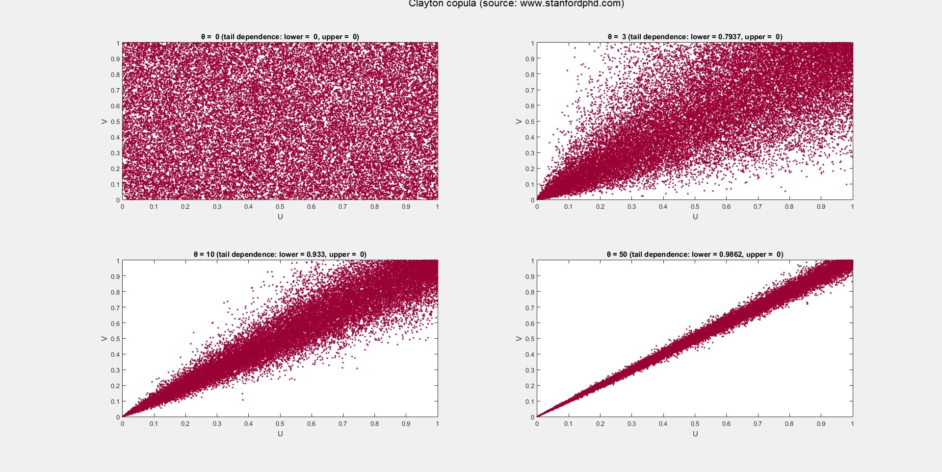
Key Properties:
- Dependence Parameter: . implies independence. As , dependence becomes perfect.
- Symmetry: It is asymmetric, favouring the lower tail.
- Tail Dependence: It has lower tail dependence but no upper tail dependence.
- Application: Perfect for modeling "joint crash" scenarios. Examples include the joint default of multiple companies during a recession, or the simultaneous sharp decline of several stock prices during a market panic.
Summary of Properties
The choice of copula is a critical modeling decision that should be driven by the phenomenon you are trying to capture. The table below summarizes the key tail dependence properties of the families we've discussed.
| Copula Family | Lower Tail () | Upper Tail () | Key Characteristic |
|---|---|---|---|
| Gaussian | 0 | 0 | No tail dependence |
| Student's t | > 0 | > 0 | Symmetric tail dependence |
| Gumbel | 0 | > 0 | Upper tail dependence only |
| Clayton | > 0 | 0 | Lower tail dependence only |
You can find a more comprehensive table, including relationships to correlation measures, in the following resource.
Copula: Modeling Nonlinear Codependence in Actuarial Science ...
The table at the end of the Stanford PhD article summarizes the key bivariate association measures for these copulas.
Review the table under section 2, focusing on the columns for lower and upper tail dependence for the Gaussian, Student, Gumbel-Hougaard, and Clayton families.
Conclusion
In this lesson, we have moved from the abstract definition of a copula to the concrete properties of specific, widely used families. We've seen that not all dependence is created equal, and the choice of copula has profound implications for risk modeling.
Key Takeaways:
- Different copula families exhibit vastly different dependence structures, which can be visualized in their scatter plots.
- The most important property for risk management is tail dependence, which quantifies the likelihood of joint extreme events.
- The Gaussian copula is tail-independent, making it risky for modeling phenomena with joint crashes or booms.
- The Gumbel copula is designed to capture upper tail dependence (joint large values).
- The Clayton copula is designed to capture lower tail dependence (joint small values).
- The Student's t-copula provides a symmetric model with dependence in both tails.
Preview of the Next Lesson
We now have a menu of copulas and an understanding of their characteristics. But how do we connect their abstract parameters (like and ) to real-world data? In the next lesson, we will explore the relationship between copula parameters and non-parametric measures of association, specifically the rank correlation coefficients Kendall's tau and Spearman's rho. This will be our first step towards calibrating and fitting copula models.