Extreme Value Theory: Estimating Quantiles and Tail Probabilities

From a Fitted GPD to VaR and ES

The POT approach gives us a model (the GPD) for the behavior of losses conditional on them exceeding the threshold $u$. To calculate a risk measure like VaR for the entire loss distribution, we need to combine this conditional tail model with information about the probability of exceeding the threshold in the first place.

Calculating VaR and ES with GPD Parameters

The probability of exceeding the threshold, $\mathrm{Pr}(X>u)$, can be estimated empirically from the data as $\frac{N_u}{n}$, where $N_u$ is the number of observations exceeding $u$ and $n$ is the total number of observations. The GPD, with its fitted parameters $\xi$ and $\beta$, models the distribution of the excesses $X-u$. By combining these two pieces, we can derive a formula for any high quantile of the original distribution.

The following resource provides the explicit formulas for VaR and ES, along with a clear, practical example. As a statistician, you'll appreciate how the formula logically combines the threshold value with a scaled term derived from the GPD's inverse CDF.

A Deeper Look at the Theory and Uncertainty

The formulas are direct, but it's crucial to understand their origin and, more importantly, the uncertainty surrounding their outputs. The video below walks through the derivation of the VaR and ES formulas from the GPD and applies them to the Danish fire insurance data we analyzed in the previous lesson. A key insight here is the discussion of the confidence intervals.

The video's final point cannot be overstated. While EVT gives us the tools to extrapolate into the far tail, the statistical uncertainty of these estimates grows immensely as we do so. A point estimate of VaR or ES is almost meaningless without an accompanying confidence interval.

Self-Assessment

To solidify your understanding, please work through the following practice problem.

Quantiles from the Block Maxima (GEV) Method

We can also estimate extreme quantiles using the GEV distribution fitted via the block maxima method. However, the interpretation is slightly different.

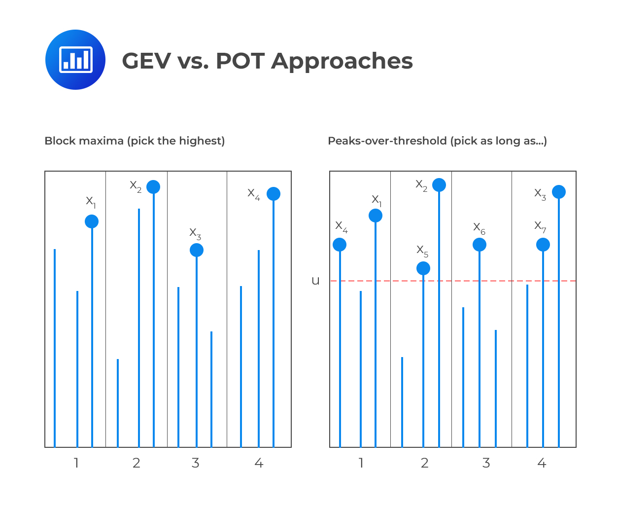
When we calculate a quantile from a fitted GEV distribution, we are finding a return level. A $t$-block return level is the value that is expected to be exceeded by the maximum of a block once every $t$ blocks. For example, if we used yearly blocks, the 100-year return level is the loss that the annual maximum loss is expected to exceed, on average, once every 100 years.

The resource below details this concept and shows how to calculate these return levels from a fitted GEV model.

While the return level is a useful measure, it is a quantile of the distribution of maxima, not of the original "parent" loss distribution. For a direct comparison with the VaR from the POT method, we need a formula that relates the GEV parameters to the quantiles of the parent distribution. The formula incorporates the block size $n$ to make this adjustment.

In practice, the POT/GPD approach is generally preferred for estimating VaR and ES because it uses data more efficiently and directly models the tail of the loss distribution.

Conclusion

This lesson concludes our exploration of Extreme Value Theory by demonstrating its ultimate purpose in risk management: the quantification of extreme events. We have connected the theoretical models (GEV and GPD) to the practical calculation of VaR and ES, the cornerstone metrics for capital adequacy and risk appetite.

Key Takeaways:

• VaR and ES from GPD: Using the fitted parameters ($\xi ,\beta$), the threshold $u$, and the empirical probability of exceeding the threshold $\frac{N_u}{n}$, we can calculate VaR and ES for any high confidence level.
• Return Levels from GEV: The GEV distribution allows us to calculate $t$-block return levels, which are quantiles of the distribution of block maxima. With an adjustment for block size, these can also be used to estimate the VaR of the underlying loss distribution.
• Uncertainty is Paramount: Estimates of extreme quantiles are subject to significant statistical uncertainty, which increases dramatically as we extrapolate further into the tail. Reporting a confidence interval is just as important as reporting the point estimate itself.
• POT vs. Block Maxima: For VaR and ES estimation, the POT approach is generally more efficient and direct, as it focuses on the distribution of all large losses rather than just the single largest loss in a period.

Preview of the Next Lesson

We have now completed our study of modeling individual risk factors, from their central tendency to their extreme tails. However, in most real-world portfolios, risks do not exist in isolation; they are interconnected. In our next module, we will turn our attention to dependence modeling. We will be introduced to copulas, a powerful statistical tool for describing and modeling the dependence structure between multiple random variables, independent of their individual marginal distributions.