Copulas for Dependent Insurance Risks

Introduction

Welcome to our final lesson on copulas. In the preceding lessons, we built our understanding from the ground up: we defined copulas using Sklar's theorem, explored various families and their properties, learned how to fit them to data, and, most recently, practiced simulating new data from these fitted models. This lesson is the capstone of the module, where we apply this entire toolkit to one of the most fundamental problems in actuarial science: quantifying the total risk of a portfolio of dependent assets or liabilities.

Our focus will be on using the simulation techniques you've learned to model the aggregate loss distribution of an insurance portfolio. From this distribution, we will calculate crucial risk measures—Value-at-Risk (VaR) and Expected Shortfall (ES)—that are the bedrock of modern economic capital and solvency regulation. By the end of this lesson, you will be able to connect the theoretical elegance of copulas to the practical necessity of managing and quantifying risk in the insurance industry.

The Challenge: Aggregating Dependent Risks

Imagine an insurer with several lines of business—for instance, term life, whole life, and disability insurance. Each line carries its own risk profile, which we can model with a marginal loss distribution. However, these risks are rarely independent. An economic downturn might increase lapse rates across all products, or a pandemic could simultaneously increase mortality and morbidity claims.

Actuaries cannot simply analyze each risk in a "silo" and sum the results. The dependence between risks significantly impacts the behavior of the total portfolio loss, especially in the tails of the distribution where extreme events occur. The total loss, $S = L_{1} + L_{2} + \dots + L_{d}$ , where $L_{i}$ is the loss from line of business $i$ , has a distribution that is notoriously difficult to determine analytically when the $L_{i}$ are dependent.

This is where copulas and Monte Carlo simulation provide a powerful solution. To start, let's explore why actuaries love copulas for this exact purpose.

Introduction to Copulas

This video segment from "Introduction to Copulas" by MJ the Fellow Actuary gives an excellent high-level overview of the practical need for copulas in risk aggregation.

Please watch the section on actuarial applications. The speaker explains how actuaries use copulas to combine different risk profiles (e.g., market, credit, operational) and why this is superior to using standard multivariate distributions. Pay attention to the discussion of capturing tail dependence, particularly with the Gumbel and normal copulas in the context of the 2008 financial crisis.

The Copula-Based Risk Modeling Workflow

The process of quantifying portfolio risk using copulas follows a systematic workflow. It integrates the skills you've acquired over the last few lessons into a coherent, practical procedure.

Model the Marginals: For each individual risk $L_{i}$ in the portfolio, fit an appropriate marginal probability distribution. This often involves using distributions we've seen before, like the Lognormal, Pareto, or Gamma, and fitting them to historical data using methods like Maximum Likelihood Estimation.
Model the Dependence: Select and fit a copula to model the joint dependence structure of the risks. This involves transforming the historical data for each risk into uniform variables (using their empirical or fitted marginal CDFs) and then fitting a copula (e.g., Gaussian, t, Gumbel) to these uniforms to estimate the dependence parameters.
Simulate Scenarios: Generate a large number ( $N$ ) of simulated scenarios for the vector of dependent losses $(L_{1}, \dots, L_{d})$ . This is done using the two-step algorithm from our previous lesson:
a. Simulate $(u_{1}, \dots, u_{d})$ from the fitted copula.
b. Transform to the target losses using the inverse CDFs of the fitted marginals: $L_{i} = F_{i}^{- 1} (u_{i})$ .
Aggregate Losses: For each of the $N$ simulated scenarios, calculate the total portfolio loss: $S_{j} = \sum_{i = 1}^{d} L_{i, j}$ for $j = 1, \dots, N$ . This gives you a large sample from the unknown distribution of $S$ .
Quantify Risk: Calculate risk measures from the empirical distribution of the simulated total losses ${S_{1}, \dots, S_{N}}$ .

The following research paper from the Society of Actuaries provides an excellent, detailed case study of this exact workflow being used to calculate economic capital for a life insurance company.

[PDF] Copula Models of Economic Capital for Life Insurance Companies

This paper demonstrates a complete, practical application of the concepts we are discussing. It walks through modeling asset and liability risks to determine the required capital.

Please read through the following parts of the paper: Section 1, "Project Objectives": Read the first few paragraphs to understand the goal. Note the explicit mention of using a copula approach to estimate economic capital via VaR and TVaR (which is the same as ES). Section 2.4, "Copula Model of the Joint Distribution": Skim this section to see how they consider different copula families. Note the discussion of elliptical and Archimedean copulas, which should be familiar. Section 3.4 and Section 4: Read these sections more carefully. This is the heart of the application. Notice how they use the AIC to select the best-fitting copula. Observe the practical challenge of building the full correlation matrix. The asset-asset correlations are estimated from data, but other correlations are supplemented with expert judgment—a common practice. Follow the description of the simulation process in Section 4.1, "Simulation from Copula", which uses the chosen t-copula and the full correlation matrix to generate scenarios. Finally, look at Section 5.2, "Example of EC Calculation", to see the final output. They use the simulated portfolio gains/losses to estimate VaR and TVaR, which is the final quantification of risk.

From Simulation to Risk Measures: VaR and ES

Once we have our $N$ simulated total portfolio losses, $S_{1}, \dots, S_{N}$ , we can estimate our risk measures.

Value-at-Risk (VaR)
The VaR at a confidence level $α$ (e.g., 99.5%) is the loss value that we are $α$ % confident will not be exceeded. It is simply the $α$ -quantile of the loss distribution.
$VaR_{α} (S) = F_{S}^{- 1} (α)$
To estimate it from our simulation, we sort the total losses in ascending order. $VaR_{α}$ is the value at the $(N \times α)$ -th position. For example, with 10,000 simulations, $VaR_{0.995}$ is the 9,950th sorted loss value.

Expected Shortfall (ES)
Also known as Conditional Tail Expectation (CTE) or Tail Value-at-Risk (TVaR), ES at level $α$ answers the question: "If we have a bad day (i.e., a loss exceeding our VaR), what is our expected loss?" It is the average of all losses in the worst $(1 - α)$ % of cases.
$ES_{α} (S) = E [S ∣ S > VaR_{α} (S)]$
We estimate ES by taking the average of all simulated losses that are greater than our estimated $VaR_{α}$ . Given your background in probability, you'll appreciate that ES is a coherent risk measure (unlike VaR, which isn't always subadditive) and provides a more complete picture of tail risk.

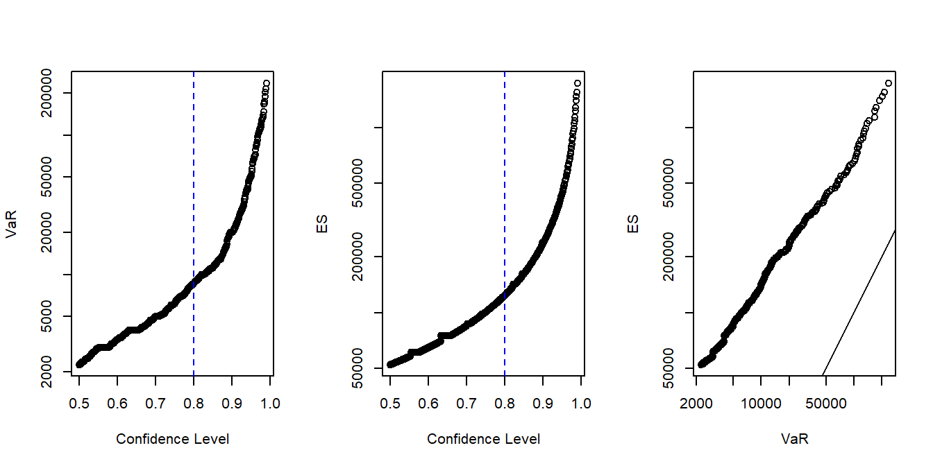
The image below illustrates these concepts. The first two plots show how VaR and ES change with the confidence level. The third plot shows ES as a function of VaR, highlighting that ES is always greater than VaR.

Plots illustrating Value-at-Risk (VaR) and Expected Shortfall (ES). The left and middle plots show VaR and ES versus the confidence level. The right plot shows ES versus VaR, demonstrating that for any given confidence level, the expected loss in the tail (ES) is greater than the threshold itself (VaR).

The Diversification Benefit

A key reason for this sophisticated modeling is to correctly capture the diversification benefit. If risks are not perfectly correlated, combining them in a portfolio reduces the overall risk relative to the sum of their individual risks. The "silo" approach, which might calculate the VaR for each line of business and simply add them up, ignores this effect and overestimates the total risk, leading to inefficient capital allocation.

Copula models allow us to quantify this benefit precisely.

[PDF] Dependent Loss Reserving Using Copulas

This paper provides a clear analysis of how dependency modeling impacts risk capital calculations, directly contrasting the silo method with a copula-based approach.

Please read the section titled "5. Risk Capital Implication". The core of this section is Table 10. Examine it closely. It compares risk measures (VaR and CTE/ES) calculated three ways: Silo: The risk of each line of business is calculated, and the results are summed. Product Copula: Assumes independence between the lines of business. Gaussian Copula: Models the actual (negative, in this case) dependence. Notice that the risk capital required under the Gaussian Copula model is less than that required under the Silo method. The difference represents the diversification benefit. This demonstrates why ignoring dependence leads to overly conservative and inefficient capital reserves.

The diversification benefit can be formally stated. For a subadditive risk measure $ρ$ like Expected Shortfall, we have:

ρ (L_{1} + L_{2}) \leq ρ (L_{1}) + ρ (L_{2})

The copula-based simulation allows us to calculate the true value of $ρ (L_{1} + L_{2})$ on the left-hand side, whereas the silo method approximates it with the larger right-hand side.

The images below provide a visual intuition for the inputs to this process. The scatterplots show data simulated from a t-copula with different dependence parameters. The histograms show the standard normal marginals. Our workflow takes these dependent points, transforms them to the desired insurance loss marginals (e.g., skewed and heavy-tailed), and then sums them to find the portfolio loss distribution.

Scatterplots and marginal histograms of samples from a bivariate t-copula with standard normal marginals. The plots show different dependence structures based on the correlation parameter (p) and degrees of freedom (df). Left: no correlation (p=0). Middle: strong positive correlation with heavy tails (p=0.8, df=1). Right: moderate positive correlation (p=0.8, df=99). This illustrates the dependent uniform variables that form the input to our simulation, before transformation to the actual loss distributions.

Conclusion

In this lesson, you have consolidated your knowledge of copulas by applying them to a complete, practical, and crucial actuarial task. You have seen how to move from individual risk models to a holistic portfolio view, using simulation to derive the aggregate loss distribution and quantify the total risk with industry-standard measures.

Key Takeaways:

Copulas are the engine for modeling the risk of a portfolio of dependent liabilities or assets.
The workflow involves modeling marginals, modeling the dependence with a copula, simulating scenarios, aggregating losses, and calculating risk measures.
Value-at-Risk (VaR) and Expected Shortfall (ES) are the primary tools for quantifying risk from the simulated aggregate loss distribution.
Modeling dependence correctly allows actuaries to quantify the diversification benefit, leading to more accurate and efficient capital management compared to the naive "silo" approach.

Preview of the Next Module

This concludes our module on copulas. You are now equipped with a sophisticated tool for dependence modeling. Our next module, Collective Risk and Ruin Theory, builds directly on these ideas. We will examine the financial health of an insurer over time, considering both incoming premiums and outgoing claims. The aggregate claim models we've just studied will be a key component. We will also explore how reinsurance can be used to manage the tail risk that you now know how to quantify, and what impact it has on an insurer's probability of ruin.

Recommended resources