Simulating Dependent Random Variables with Copulas

Introduction

In our previous lesson, we focused on fitting a copula model to data using maximum likelihood estimation. This allowed us to select an appropriate copula family and estimate its parameters, effectively capturing the underlying dependence structure. Now that we have a fully specified model, we can move from describing dependence to actively using it.

This lesson addresses the logical next step: simulating new data from our fitted model. You will learn the general algorithm for generating pairs of dependent random variables that follow a specific copula structure and desired marginal distributions. This skill is the engine of Monte Carlo simulation for dependent risks, a cornerstone of modern actuarial science used for everything from pricing complex derivatives to calculating economic capital.

The Fundamental Simulation Algorithm

The process of simulating dependent variables $(X_{1}, X_{2})$ is elegantly broken down into two main steps, a direct application of Sklar's theorem and the probability integral transform you are familiar with from your statistics background.

Simulate from the Copula: Generate a pair of dependent random variables $(u_{1}, u_{2})$ from the chosen copula $C$ . These variables are, by definition, uniformly distributed on $[0, 1]$ and contain the desired dependence pattern.
Transform to the Marginals: Use the inverse cumulative distribution functions (CDFs), or quantile functions, of the desired marginal distributions to transform the uniform variables into the target variables: $X_{1} = F_{1}^{- 1} (u_{1}) and X_{2} = F_{2}^{- 1} (u_{2})$

The pair $(X_{1}, X_{2})$ will now have the marginal distributions $F_{1}$ and $F_{2}$ respectively, and their dependence structure will be governed by the copula $C$ . This is because the inverse CDF transform ensures the correct marginals, while the dependence is carried over from the initial pair $(u_{1}, u_{2})$ .

This two-step procedure is universal. The main challenge lies in Step 1, as the specific technique for generating the dependent uniform pair $(u_{1}, u_{2})$ differs between copula families.

[PDF] A Copulas-based Approach to Modeling Dependence in Decision ...

This research paper provides a clear, formal description of the inverse transformation step.

Please read the section titled "Step 4. Point-to-point inverse marginal transformation". Focus on the two key equations: the transformation formulas, and the example that follows, which shows how simulated uniform values are transformed into variables with specific Normal and Gamma distributions. This solidifies the logic of our second step.

Simulating from Elliptical Copulas: Gaussian and t-Copulas

Elliptical copulas, such as the Gaussian and t-copulas, are simulated using a method that leverages their connection to multivariate normal and t-distributions. The core tool for this is the Cholesky decomposition.

The following video provides an excellent, step-by-step walkthrough of this entire process in a spreadsheet environment, which will appeal to your preference for practical calculation.

Copulas 4 - creating simulations with copulas

This video, "Copulas 4 - creating simulations with copulas" from the channel Paul Sweeting, demonstrates the mechanics of simulating from elliptical copulas.

Please watch the following segments carefully: Gaussian Copula Simulation (Cholesky method): This is the most crucial part. The presenter explains how to: Start with a correlation matrix \Sigma. Use Cholesky decomposition to find a lower-triangular matrix L such that \Sigma = LL^T. Generate independent standard normal variables \mathbf{z}. Create correlated standard normal variables via the matrix multiplication \mathbf{x} = L\mathbf{z}. This is the key step for introducing dependence. Transforming to Uniforms (from correlated normals): After generating the correlated normal variables \mathbf{x}, this part shows how to convert them into the dependent uniform pair (u_1, u_2) required for our general algorithm. This is done by applying the standard normal CDF: u_i = \Phi(x_i). The presenter then demonstrates the second step of our algorithm: transforming these uniform variables into final variables with specified marginals (in this case, t-distributions). t-Copula Simulation (t-copula method): This segment explains the modification needed to simulate from a t-copula. The process begins similarly to the Gaussian case but includes an extra step to generate the characteristic fat tails of the t-distribution. Pay attention to the use of a chi-squared variate to scale the correlated normal variables.

Let's summarize the algorithm for simulating from a $d$ -dimensional Gaussian copula with correlation matrix $Σ$ :

Find the Cholesky decomposition $L$ of $Σ$ such that $Σ = L L^{T}$ .
Generate a vector $z = (z_{1}, \dots, z_{d})$ of $d$ independent standard normal random variables.
Calculate the vector of correlated normal variables: $x = L z$ .
Component-wise, transform $x$ into a vector of dependent uniform variables $u$ using the standard normal CDF: $u_{i} = Φ (x_{i})$ for $i = 1, \dots, d$ .
Finally, transform $u$ to the target variables using the inverse marginal CDFs: $X_{i} = F_{i}^{- 1} (u_{i})$ .

The algorithm for the t-copula is a slight modification:

Steps 1-3 are the same as for the Gaussian copula.
Generate a random variable $s$ from a chi-squared distribution with $ν$ degrees of freedom, independent of $z$ . ( $ν$ is the degrees of freedom parameter of the t-copula).
Calculate a vector of correlated t-distributed variables: $y = \frac{x}{s / ν}$ .
Transform $y$ into dependent uniform variables $u$ using the CDF of the standard t-distribution with $ν$ degrees of freedom: $u_{i} = t_{ν} (y_{i})$ .
Transform $u$ using the inverse marginal CDFs: $X_{i} = F_{i}^{- 1} (u_{i})$ .

Simulating from Archimedean Copulas

The simulation method for Archimedean copulas (like Clayton, Gumbel, Frank) is different and relies on their generator functions, $ϕ$ . The general algorithm involves generating independent uniform variables and then using a specific transformation that depends on the copula's generator. While the derivations can be complex, the resulting algorithms are often computationally efficient.

The key is to generate $u_{1}$ and then generate $u_{2}$ from the conditional distribution $C (u_{2} ∣ u_{1})$ . For many Archimedean copulas, the inverse of this conditional distribution can be expressed in a closed form, leading to a direct simulation algorithm.

For example, to simulate a pair $(u_{1}, u_{2})$ from a Clayton copula with parameter $θ$ :

Generate two independent standard uniform random variables, $v_{1}$ and $v_{2}$ .
Set $u_{1} = v_{1}$ .
Calculate $u_{2} = (v_{1}^{- θ} (v_{2}^{- θ / (1 + θ)} - 1) + 1)^{- 1/ θ}$ .

Notice that this directly gives the dependent uniform pair $(u_{1}, u_{2})$ . From here, you would proceed to Step 2 of our main algorithm: applying the inverse marginal CDFs. Similar (though different) formulas exist for other Archimedean families. You are not typically required to memorize these specific formulas for the CS2 exam, but you should understand that a specific algorithm exists for each family.

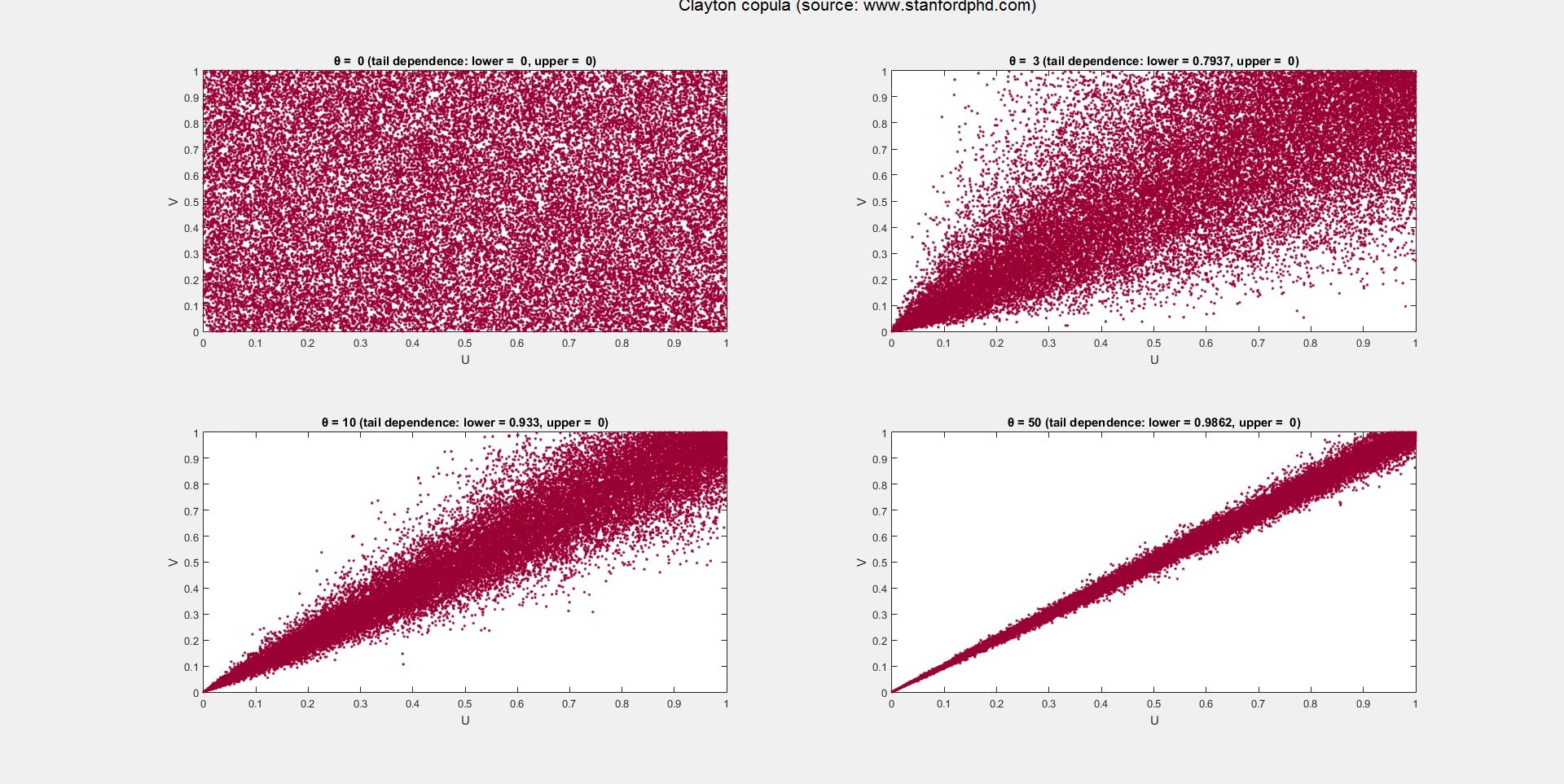
The images below show scatter plots of 1000 points simulated from various copula families. This is the visual output of the algorithms we've discussed. Notice how the Clayton copula concentrates points in the lower-left tail, while the Gumbel concentrates them in the upper-right, reflecting their different tail dependence properties.

Simulated data from four different copula families: Gaussian, t-Copula, Clayton, and Gumbel. Each plot illustrates a distinct dependence structure.

Simulations from a Clayton copula with increasing parameter $\theta$. As $\theta$ increases, the lower-tail dependence becomes stronger.

Conclusion

You are now equipped with the fundamental knowledge to simulate dependent risks, a critical tool in the actuarial toolkit. By combining a method to generate dependent uniform variables with the inverse transform method for the marginals, you can construct sophisticated Monte Carlo simulations for a wide array of problems.

Key Takeaways:

Simulation of dependent variables is a two-step process: (1) simulate a dependent uniform pair $(u_{1}, u_{2})$ from the chosen copula, and (2) transform this pair into the target variables $(X_{1}, X_{2})$ using their respective inverse CDFs.
The method for Step 1 depends on the copula family.
Elliptical copulas (Gaussian, t) are simulated using Cholesky decomposition of the correlation matrix to create correlated normal variables, which are then transformed to uniform.
Archimedean copulas (Clayton, Gumbel, Frank) are simulated using specific algorithms derived from their generator functions, often involving the conditional distribution $C (u_{2} ∣ u_{1})$ .

Preview of the Next Lesson

In our final lesson on copulas, we will put everything together. We will take a practical actuarial problem, such as modeling the aggregate claims from two dependent lines of business. We will fit a copula to historical data (as in the last lesson) and then use the simulation techniques learned today to generate a large number of scenarios for future losses. This will allow us to estimate the distribution of the total loss and calculate key risk measures like Value-at-Risk (VaR) and Tail Value-at-Risk (TVaR).