Parametric Survival Models for Mortality Rate Calculation

Introduction

In our previous lesson, we established how to calculate the complete and curtate future lifetimes, $e_{x}^{\circ}$ and $e_{x}$ , by integrating or summing a given survival function, $_{t} p_{x}$ . This process treated the survival function as a given, almost like a black box. Today, we'll open that box to explore some of the most common and powerful "laws of mortality"—specific mathematical formulas used to model the survival function itself.

This lesson focuses on applying standard parametric survival models, a cornerstone of actuarial science. You'll learn about the assumptions behind the Weibull, Gompertz, and Makeham models and how to use them to compute mortality rates and survival probabilities. For someone with your background in probability theory, this is analogous to moving from an empirical distribution to fitting a named probability distribution (like the normal or gamma) to data. These parametric forms provide a smooth, differentiable function for survival, which is invaluable for pricing, reserving, and forecasting.

The Foundation: From Hazard to Survival

All parametric survival models begin with an assumption about the shape of the hazard function, or as it's known in actuarial science, the force of mortality, $μ_{x}$ . As we've touched on before, the force of mortality at age $x$ represents the instantaneous rate of death for a person who has survived to that age.

The crucial link between the force of mortality and the probability of a person aged $x$ surviving for $t$ more years, $_{t} p_{x}$ , is given by this fundamental relationship:

_{t} p_{x} = exp (- \int_{0}^{t} μ_{x + s} d s)

This equation states that the probability of surviving from age $x$ to $x + t$ is determined by the cumulative hazard experienced over that interval. Every model we discuss today is simply a different choice for the function $μ_{x}$ .

To solidify your understanding of this core concept and its derivation, the following reading is highly recommended.

[PDF] Chapter 2 - Survival Models

This section from a University of Florida course note provides a clear definition of the force of mortality and a rigorous derivation of its relationship with the survival function.

Please read the sections titled "Force of Mortality" and the derivations that follow. Focus on the equation that expresses {}_t p_x as an exponential of an integral of \mu_{x+r} (note the use of r instead of s as the integration variable). You'll find it under this expression. This is the master formula for this lesson.

With this foundation, let's explore the models.

Model 1: The Weibull Distribution

The Weibull distribution is a versatile two-parameter model widely used in reliability engineering and also in survival analysis. Its defining feature is a hazard function that follows a power law with respect to time.

The hazard function for a newborn is given by:

μ_{t} = κ λ^{κ} t^{κ - 1} for t \geq 0

Here, $λ > 0$ is a scale parameter and $κ > 0$ is a shape parameter. The shape parameter $κ$ is particularly important as it dictates the nature of the risk over time:

$κ < 1$ : Decreasing hazard. This models situations where risk is highest at the beginning, like infant mortality or "burn-in" failures of electronic components.
$κ = 1$ : Constant hazard ( $μ_{t} = λ$ ). The Weibull distribution simplifies to the Exponential distribution, which has the "memoryless" property.
$κ > 1$ : Increasing hazard. This is the most common scenario for human mortality, representing aging and wear-and-tear.

Integrating this hazard function from 0 to $t$ gives the cumulative hazard $H (t) = (λ t)^{κ}$ , which leads to the survival function for a newborn:

S_{0} (t) = e^{- (λ t)^{κ}}

Unlike the Gompertz and Makeham laws we'll see next, the Weibull hazard depends on the time $t$ since birth, not the attained age $x$ . This means the survival probability for a life aged $x$ , $_{t} p_{x}$ , is calculated from the base survival function:

_{t} p_{x} = \frac{S _{0} ( x + t )}{S _{0} ( x )} = \frac{e ^{- (λ (x + t))^{κ}}}{e ^{- (λ x)^{κ}}} = exp (λ^{κ} [x^{κ} - (x + t)^{κ}])

Notice that the future lifetime distribution of a life aged $x$ is not itself a Weibull distribution.

[PDF] Chapter 4: Probability Models in Survival Analysis - Mathematics

This excerpt from "Probability Models in Survival Analysis" by Leemis provides a thorough introduction to the Weibull distribution.

Please read the section titled "Weibull Distribution". Pay close attention to the definitions of the survivor and hazard functions, and the explanation of the role of the shape parameter \kappa.

Model 2: The Gompertz Law

Published in 1825, the Gompertz law is one of the earliest and most enduring models of human mortality. It is based on the empirical observation that a person's resistance to death decreases as they age. This is mathematically formulated as a force of mortality that increases exponentially with age:

μ_{x} = B C^{x}

where $B > 0$ and $C > 1$ are constants. $B$ represents the baseline mortality at age 0, and $C$ controls the rate of aging.

To find the survival probability $_{t} p_{x}$ , we apply our master formula:

_{t} p_{x} = exp (- \int_{0}^{t} μ_{x + s} d s) = exp (- \int_{0}^{t} B C^{x + s} d s)

= exp (- B C^{x} \int_{0}^{t} C^{s} d s)

The integral evaluates to $\int_{0}^{t} C^{s} d s = [\frac{C ^{s}}{l n C}]_{0}^{t} = \frac{C ^{t} - 1}{l n C}$ . Substituting this back gives the survival function under Gompertz's law:

_{t} p_{x} = exp (- \frac{B C ^{x}}{ln C} (C^{t} - 1))

Model 3: The Makeham Law

In 1860, William Makeham proposed a modification to Gompertz's law to better fit population data. He added a constant term, $A$ , to the force of mortality:

μ_{x} = A + B C^{x}

The genius of this addition lies in its interpretation: the risk of death is composed of two parts. The $B C^{x}$ term is the Gompertz component, representing death due to aging. The constant $A$ represents a component of mortality that is independent of age, often interpreted as death from accidents or other causes not related to senescence.

Calculating the survival probability follows the same process, and the structure of $μ_{x}$ leads to an elegant result:

_{t} p_{x} = exp (- \int_{0}^{t} (A + B C^{x + s}) d s)

= exp (- \int_{0}^{t} A d s - \int_{0}^{t} B C^{x + s} d s) = exp (- A t) \cdot exp (- \int_{0}^{t} B C^{x + s} d s)

We immediately recognize the second term as the survival probability under Gompertz's law. Therefore, under Makeham's law:

_{t} p_{x} = e^{- A t} \cdot exp (- \frac{B C ^{x}}{ln C} (C^{t} - 1))

This shows that survival under Makeham's law is the product of an age-independent survival probability ( $e^{- A t}$ ) and an age-dependent Gompertz survival probability.

The following video provides an excellent summary and derivation for all the models discussed.

Survival Models Concepts

This video, "Survival Models Concepts," walks through the derivation of the survival functions for the Weibull, Gompertz, and Makeham models starting from their hazard functions.

I recommend you watch the following segments: Weibull Model: This part covers the derivation of the hazard and survival functions. Gompertz Law: This segment shows the step-by-step calculation of {}_t p_x. Makeham Law: Here, the derivation elegantly builds upon the Gompertz result.

Visualizing and Applying the Models

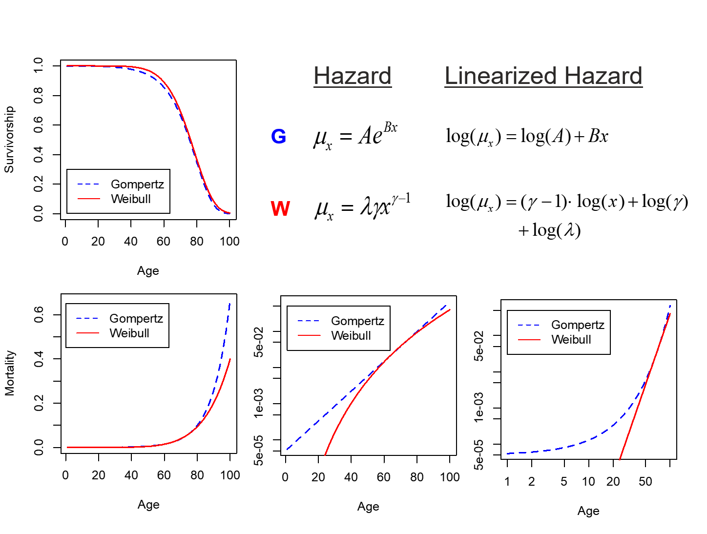
The choice of model depends on how well its assumed hazard shape fits the data. The Gompertz and Weibull models, while both capable of modeling increasing hazard, have distinct shapes.

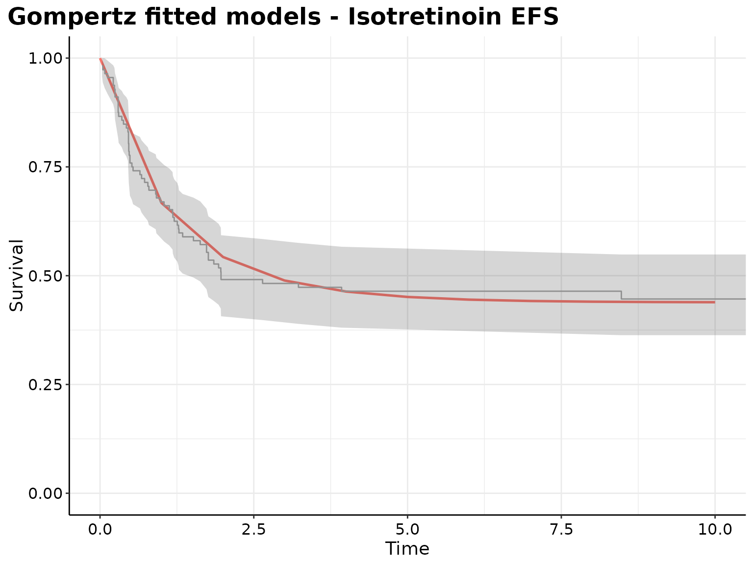
This figure compares the survivorship, mortality, and hazard functions for Gompertz and Weibull models. Note the different curvatures. The "Linearized Hazard" plots show how transforming the axes can reveal if data fits a particular model (a straight line suggests a good fit).

In practice, these models are fitted to real-world data to estimate the parameters.

This plot shows a Gompertz survival model (red line) fitted to Kaplan-Meier survival data (black steps) for patients in a clinical trial. The shaded area represents the confidence interval. This demonstrates how a smooth parametric curve can summarize noisy, real-world survival data.

Worked Example: Applying Makeham's Law

Let's solve a problem. A certain population's mortality is modeled by Makeham's law with $μ_{x} = A + B C^{x}$ , where $A = 0.00022$ , $B = 2.7 \times 1 0^{- 5}$ , and $C = 1.124$ .

Calculate the probability that a person aged 60 survives for at least 5 years.

Solution:
We need to calculate $_{5} p_{60}$ .
First, let's find the value of the Gompertz component's constant term: $\frac{B}{l n C}$ .
$ln C = ln (1.124) \approx 0.1169$ .
So, $\frac{B}{l n C} = \frac{2.7 \times 1 0 ^{- 5}}{0.1169} \approx 0.0002309$ .

Now, we use the formula for $_{t} p_{x}$ with $x = 60$ and $t = 5$ :

_{5} p_{60} = exp (- 5 A) \cdot exp (- \frac{B C ^{60}}{ln C} (C^{5} - 1))

Let's calculate the components:

$- 5 A = - 5 \times 0.00022 = - 0.0011$
$C^{5} = (1.124)^{5} \approx 1.793$
$C^{60} = (1.124)^{60} \approx 406.45$
The argument of the second exponential is:
$- (\frac{B C ^{60}}{l n C} (C^{5} - 1)) = - (0.0002309 \times 406.45) \times (1.793 - 1)$
$= - (0.09386) \times (0.793) \approx - 0.07442$

Combining these parts:

_{5} p_{60} = e^{- 0.0011} \times e^{- 0.07442} = e^{- 0.07552} \approx 0.9272

So, the probability that a person aged 60 survives to age 65 is approximately 92.72%.

Conclusion

In this lesson, we moved from abstract survival functions to concrete, named models that describe mortality patterns. By defining a specific functional form for the force of mortality ( $μ_{x}$ ), we can derive corresponding formulas for survival probabilities and other actuarial quantities.

Key Takeaways:

Parametric models are defined by the mathematical form of their hazard function (force of mortality).
The survival probability $_{t} p_{x}$ is found by integrating the force of mortality via the formula $_{t} p_{x} = exp (- \int_{0}^{t} μ_{x + s} d s)$ .
Weibull model: The hazard is a power function of time, $μ_{t} \propto t^{κ - 1}$ . It's flexible and can model decreasing, constant (exponential), or increasing hazard.
Gompertz law: The hazard grows exponentially with age, $μ_{x} = B C^{x}$ . It's a classic model for aging.
Makeham law: An extension of Gompertz, $μ_{x} = A + B C^{x}$ , which adds a constant risk factor to account for accidental or age-independent death.

In our next lesson, we will build upon these concepts to solve problems involving more complex survival periods, such as temporary and deferred probabilities, which are essential for pricing insurance products like term life insurance and endowments.

Recommended resources