Deferred & Temporary Survival Probabilities

Introduction

In our last session, we explored how to derive survival probabilities from parametric models like Gompertz and Makeham. We focused on calculating $_{t} p_{x}$ , the probability that a person aged $x$ survives for at least $t$ more years. Today, we will use this fundamental probability as a building block to construct and solve problems involving more specific time windows.

This lesson will introduce you to temporary and deferred probabilities, which are essential for partitioning an individual's future lifetime into periods of interest. You will learn the standard actuarial notation for these concepts and, more importantly, how to calculate them. We will also tackle a common practical challenge: calculating probabilities for non-integer time periods (e.g., surviving for 6 months). This requires making assumptions about how deaths are distributed throughout a year, and we will explore the two most common methods: the Uniform Distribution of Deaths (UDD) and Constant Force of Mortality (CFM).

Your background in probability theory will be particularly useful here, as we can frame these actuarial concepts in terms of the cumulative distribution function and conditional probabilities of the future lifetime random variable, $T_{x}$ .

Defining Probabilities of Death and Deferral

Let's begin by formally defining the key probabilities we'll be working with. While $_{t} p_{x}$ represents survival, its complement, $_{t} q_{x}$ , represents mortality. From there, we can define probabilities for periods that are deferred into the future.

The image below provides a clear visual representation of the three main types of probabilities associated with the future lifetime of a person currently aged $x$ .

This diagram illustrates the time intervals for three fundamental probabilities: survival over a period $t$ (${}_t p_x$), mortality within a period $t$ (${}_t q_x$), and deferred mortality within a period $u$ after a deferral of $t$ years (${}_{t|u} q_x$).

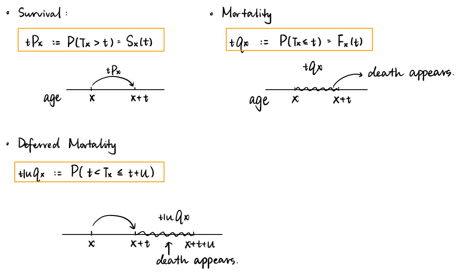
1. Temporary Mortality Probability: $_{t} q_{x}$

This is the probability that a person aged $x$ will die within the next $t$ years. From a probabilistic standpoint, if $T_{x}$ is the random variable for the future lifetime of (x), then:

_{t} q_{x} = P (T_{x} \leq t)

This is simply the cumulative distribution function (CDF) of $T_{x}$ . Since a person must either survive for $t$ years or die within $t$ years, we have the fundamental relationship:

_{t} p_{x} +_{t} q_{x} = 1

Therefore, once you calculate a survival probability using a parametric model or a life table, finding the corresponding mortality probability is straightforward: $_{t} q_{x} = 1 -_{t} p_{x}$ .

2. Deferred Mortality Probability: $_{n ∣ m} q_{x}$

This is the probability that a person aged $x$ will survive for $n$ years and then die within the following $m$ years. In terms of $T_{x}$ , this is:

_{n ∣ m} q_{x} = P (n < T_{x} \leq n + m)

We can calculate this by considering the difference between two survival probabilities. The event $n < T_{x} \leq n + m$ is equivalent to the event $(T_{x} > n)$ minus the event $(T_{x} > n + m)$ . Therefore:

_{n ∣ m} q_{x} = P (T_{x} > n) - P (T_{x} > n + m) =_{n} p_{x} -_{n + m} p_{x}

Alternatively, we can think of this conditionally. The person must first survive $n$ years (with probability $_{n} p_{x}$ ), and then, having reached age $x + n$ , must die within the next $m$ years (with probability $_{m} q_{x + n}$ ). This gives us a second, equally important identity:

_{n ∣ m} q_{x} =_{n} p_{x} \cdot_{m} q_{x + n}

A special case is a deferred whole life probability, $_{n} q_{x}$ , which is the probability of dying any time after $n$ years. This is simply the probability of surviving $n$ years: $_{n} q_{x} = P (T_{x} > n) =_{n} p_{x}$ .

The following video provides a thorough walkthrough of these concepts, starting from the definition of the future lifetime random variable, which should align well with your statistical background.

4.4. Actuarial Math: Survival Models D

This video, "Actuarial Math: Survival Models D," introduces the future lifetime variable T_x and uses it to formally define the survival and mortality probabilities {}_t p_x and {}_t q_x.

Please watch the first two main segments: Future Lifetime and {}_t p_x: This part defines the remaining lifetime T_x and derives the expression for {}_t p_x as S(x+t)/S(x). Mortality Probability {}_t q_x: This segment introduces the notation {}_t q_x and shows its relationship to {}_t p_x and the underlying survival function S(x).

Dealing with Fractional Ages

The formulas above work perfectly for integer values of $t$ , $n$ , and $m$ . However, in practice, we often need to calculate probabilities for parts of a year, for instance, for an insurance policy with a monthly premium or a 3-month waiting period. This requires an assumption about how deaths are distributed within each year of age.

Assumption 1: Uniform Distribution of Deaths (UDD)

The UDD assumption states that for any integer age $x$ , the number of deaths between age $x$ and $x + 1$ is distributed uniformly over that year.
If $l_{x}$ is the number of people alive at age $x$ and $d_{x}$ is the number of deaths between $x$ and $x + 1$ , this means the number of survivors at a fractional age $x + s$ (where $0 \leq s \leq 1$ ) is found by linear interpolation:

l_{x + s} = l_{x} - s \cdot d_{x} = l_{x} (1 - s \cdot q_{x})

From this, we can derive key probability formulas. For a period $s$ where $0 \leq s \leq 1$ :

Mortality within the first part of a year: The probability of dying within the first fraction $s$ of the year is simply proportional to $s$ . $_{s} q_{x} = \frac{l _{x} - l _{x + s}}{l _{x}} = \frac{s \cdot d _{x}}{l _{x}} = s \cdot q_{x}$
Mortality in a future part of a year: The probability of dying in a period of length $s$ after already surviving a period of length $t$ (where $s + t \leq 1$ ) is more complex. This is a conditional probability. $_{s} q_{x + t} = P (T_{x} \in (t, t + s] ∣ T_{x} > t) = \frac{P ( T _{x} \in ( t , t + s ])}{P ( T _{x} > t )} = \frac{_{t + s} q _{x} - _{t} q _{x}}{_{t} p _{x}} = \frac{( t + s ) q _{x} - t q _{x}}{1 - t q _{x}} = \frac{s q _{x}}{1 - t q _{x}}$

This last formula is crucial. Notice that as $t$ increases (as you get older within the year), the denominator decreases, so the probability of death $_{s} q_{x + t}$ increases. This makes sense: under UDD, the number of deaths is constant over time, but the population at risk is shrinking, so the rate of death must increase.

[PDF] Contents - Actuarial Study Materials

This section from the ASM study manual provides a detailed, practical guide to calculations under UDD.

Please read the subsection "Uniform distribution of deaths". Focus on understanding formula (7.2), sqx = sqx, and the more general and important formula (7.3), sqx+t. Then, work through Example 7A carefully, as it's a direct application of this formula.

Assumption 2: Constant Force of Mortality (CFM)

The CFM assumption states that the force of mortality, $μ$ , is constant between any two integer ages. So, for $0 < s \leq 1$ , we have $μ_{x + s} = μ_{x}$ .
Recall from our previous lesson the fundamental relationship:

_{s} p_{x} = exp (- \int_{0}^{s} μ_{x + r} d r)

Under CFM, this integral simplifies beautifully:

_{s} p_{x} = exp (- μ_{x} \cdot s)

Since for a full year $_{1} p_{x} = p_{x} = e^{- μ_{x}}$ , we can also write $μ_{x} = - ln (p_{x})$ . Substituting this back gives the most common form for CFM calculations:

_{s} p_{x} = exp (s \cdot ln (p_{x})) = (p_{x})^{s}

The key feature of CFM is that the survival probability over a fraction of a year depends only on the length of that fraction, not on when it occurs during the year. That is, for $s + t \leq 1$ :

_{s} p_{x + t} = (p_{x})^{s}

This makes calculations under CFM significantly simpler than under UDD.

Chapter 3 The Life Table

This video, "Chapter 3 The Life Table," offers a great visual and verbal explanation contrasting the UDD and CFM assumptions for handling non-integer ages.

Please watch the two key segments on this topic: UDD: This section provides an intuitive explanation and a worked example that highlights why {}_s q_{x+t} is not simply s \cdot q_x. The diagram at the end is very helpful. CFM: This section explains the CFM assumption and contrasts it directly with UDD, emphasizing the simplicity of the resulting formulas.

Worked Example: UDD vs. CFM

Let's put this all together. Suppose you are given that for a life aged 50, the mortality rate for the year is $q_{50} = 0.04$ . Calculate the probability that this person, having reached age 50.25, dies within the next 6 months (i.e., before age 50.75). We want to find $_{0.5} q_{50.25}$ .

1. Under UDD:
We use the formula $_{s} q_{x + t} = \frac{s q _{x}}{1 - t q _{x}}$ with $x = 50$ , $s = 0.5$ , and $t = 0.25$ .

_{0.5} q_{50.25} = \frac{0.5 \times q _{50}}{1 - 0.25 \times q _{50}} = \frac{0.5 \times 0.04}{1 - 0.25 \times 0.04} = \frac{0.02}{1 - 0.01} = \frac{0.02}{0.99} \approx 0.0202

2. Under CFM:
First, we find the one-year survival probability: $p_{50} = 1 - q_{50} = 1 - 0.04 = 0.96$ .
Under CFM, the probability of surviving for any period $s$ within the year is $(p_{50})^{s}$ . The probability of dying is $1 - (p_{50})^{s}$ .
We are interested in a period of length 0.5 years. The probability of death is independent of the starting age (50.25) within the year.

_{0.5} q_{50.25} = 1 -_{0.5} p_{50.25} = 1 - (p_{50})^{0.5} = 1 - (0.96)^{0.5} \approx 1 - 0.9798 = 0.0202

In this specific case, the results are very similar, but this is not always true. The difference between the two assumptions becomes more pronounced as the mortality rate $q_{x}$ gets larger.

For additional practice, I highly recommend working through some of the exercises in the ASM manual. For example, try Exercise 7.3 and 7.4, which involve durations crossing an integer boundary, and Exercise 7.23, which directly compares UDD and CFM. The solutions are provided in the document for you to check your work.

[PDF] Contents - Actuarial Study Materials

This resource contains practice problems and solutions that will help you master calculations involving UDD and CFM.

I suggest you attempt Exercises 7.3 and 7.4 under the "Uniform distribution of death" section. Then, try Exercise 7.23 under the "Constant force of mortality" section. You can verify your answers using the solutions section that begins on page 141.

Conclusion

This lesson has equipped you with the tools to calculate fundamental actuarial probabilities for specific time windows, both integer and fractional. These are not just theoretical exercises; they form the basis for pricing and reserving for real-world insurance products.

Key Takeaways:

Temporary mortality ( $_{t} q_{x}$ ) and deferred mortality ( $_{n ∣ m} q_{x}$ ) are defined in terms of the future lifetime random variable $T_{x}$ and can be calculated from survival probabilities ( $_{t} p_{x}$ ).
The key identity for deferred mortality is $_{n ∣ m} q_{x} =_{n} p_{x} -_{n + m} p_{x}$ .
Calculating probabilities for fractional ages requires an assumption about the distribution of deaths within a year.
UDD (Uniform Distribution of Deaths) assumes a constant number of deaths over the year, leading to the formula $_{s} q_{x + t} = \frac{s q _{x}}{1 - t q _{x}}$ .
CFM (Constant Force of Mortality) assumes a constant rate of death over the year, leading to the simpler formula $_{s} p_{x} = (p_{x})^{s}$ .

In the upcoming lessons, we will shift our focus from using pre-defined models to the statistical problem of estimating survival functions from observed data. This will introduce you to the concepts of censoring and non-parametric estimation methods like the Kaplan-Meier estimator, bringing us closer to the work of a practicing statistician or actuary.

Recommended resources