Building a Generator Matrix from Transition Rates

From Transition Probabilities to Transition Rates

You'll recall from your study of discrete-time Markov chains that the process is governed by a transition probability matrix, $\mathsf{P}$, where $P_{ij}$ gives the probability of moving from state $i$ to state $j$ in exactly one time step.

In a continuous-time process, the notion of a "single time step" disappears. Jumps can happen at any instant. This fundamentally changes our perspective:

• Instead of asking for the probability of a jump in a fixed interval, we define an instantaneous rate of transition.
• The time spent in any given state before a jump occurs, known as the holding time, becomes a random variable. For the Markov property (the "memorylessness") to hold, these holding times must follow an exponential distribution.

The following video provides a formal introduction to Continuous-Time Markov Chains (CTMCs), defining them as "pure jump processes" and highlighting the crucial role of exponentially distributed holding times.

The Generator Matrix, $\mathsf{Q}$

The entire dynamics of a time-homogeneous CTMC can be summarized by a single matrix: the generator matrix $\mathsf{Q}$. This matrix is built from the infinitesimal transition rates, $q_{ij}$, which represent the instantaneous rate at which the process jumps from state $i$ to state $j$.

Here is the fundamental definition for constructing the generator matrix:

• Off-diagonal elements ($i\ne j$): The entry $q_{ij}$ is the transition rate from state $i$ to state $j$. These rates are always non-negative ($q_{ij}\ge 0$). If $q_{ij}=0$, it means a direct transition from $i$ to $j$ is impossible.
• Diagonal elements ($i=j$): The entry $q_{ii}$ is defined such that each row of the matrix sums to zero. Therefore: $$q_{ii}=-\sum _{j\ne i}{q}_{ij}$$

This structure leads to three key properties of any generator matrix:

1. Off-diagonal elements are non-negative ($q_{ij}\ge 0$ for $i\ne j$).
2. Diagonal elements are non-positive ($q_{ii}\le 0$).
3. The sum of the elements in each row is exactly zero.

Interpretation of the Elements

The elements of $\mathsf{Q}$ have a clear, intuitive meaning:

• $q_{ij}$ (for $i\ne j$) is the rate of jumping from state $i$ to state $j$.
• $-q_{ii}$ represents the total rate of leaving state $i$ for any other state. We often denote this total exit rate as $q_i=-q_{ii}$. This rate will become critically important in our next lesson when we discuss holding time distributions in more detail.

The following reading provides a concise and practical guide to defining and interpreting the generator matrix.

Constructing $\mathsf{Q}$ from a Rate Diagram

In practice, we often start with a rate diagram, which is a directed graph where nodes represent the states and arrows represent possible transitions, labeled with their corresponding rates. Constructing the generator matrix from such a diagram is a straightforward process.

Let's consider the following three-state model:

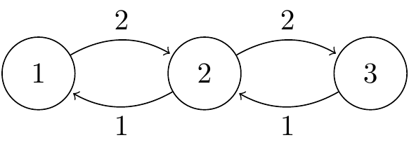
To construct the 3x3 generator matrix $\mathsf{Q}$, we follow the rules row by row:

• Row 1 (State 1):

  • There is one outgoing arrow, from state 1 to state 2, with rate 2. So, $q_{12}=2$.
  • There is no arrow from 1 to 3, so $q_{13}=0$.
  • The diagonal element is $q_{11}=-(q_{12}+q_{13})=-(2+0)=-2$.
  • Row 1 is: $[-2,2,0]$

• Row 2 (State 2):

  • There is an arrow from state 2 to state 1 with rate 1, so $q_{21}=1$.
  • There is an arrow from state 2 to state 3 with rate 2, so $q_{23}=2$.
  • The diagonal element is $q_{22}=-(q_{21}+q_{23})=-(1+2)=-3$.
  • Row 2 is: $[1,-3,2]$

• Row 3 (State 3):

  • There is an arrow from state 3 to state 2 with rate 1, so $q_{32}=1$.
  • There is no arrow from 3 to 1, so $q_{31}=0$.
  • The diagonal element is $q_{33}=-(q_{31}+q_{32})=-(0+1)=-1$.
  • Row 3 is: $[0,1,-1]$

Putting it all together, the generator matrix is:

This exact example is worked through in the resource you just reviewed. Let's now apply this method to a few more examples, including one in a classic actuarial context.

Notice how the Poisson process with rate $\lambda$ can be described as a CTMC on the states $\{0,1,2,\dots \}$ where jumps only occur from state $i$ to $i+1$ with rate $\lambda$. This provides a satisfying connection back to the topics from our previous module.

An Actuarial Example: The Healthy-Sick-Dead Model

A cornerstone of actuarial modeling is the multi-state model for life insurance and pensions. A simple but powerful version is the "Healthy-Sick-Dead" model.

Let's analyze the transitions shown in the diagram:

• A healthy person becomes sick at rate $\sigma$.
• A healthy person dies at rate $\mu$.
• A sick person recovers and becomes healthy at rate $\rho$.
• A sick person dies at rate $\nu$.
• The "Dead" state is an absorbing state: there are no outgoing arrows. Once the process enters this state, it stays there forever.

Let's construct the generator matrix $\mathsf{Q}$ for this model, with states ordered (H, S, D).

• Row H (Healthy):
  • Outgoing rate to S is $\sigma$, so $q_{HS}=\sigma$.
  • Outgoing rate to D is $\mu$, so $q_{HD}=\mu$.
  • Diagonal element is $q_{HH}=-(\sigma +\mu )$.
• Row S (Sick):
  • Outgoing rate to H is $\rho$, so $q_{SH}=\rho$.
  • Outgoing rate to D is $\nu$, so $q_{SD}=\nu$.
  • Diagonal element is $q_{SS}=-(\rho +\nu )$.
• Row D (Dead):
  • There are no outgoing transitions. All rates are 0.
  • Diagonal element is $q_{DD}=-(0)=0$.

The complete generator matrix is:

The matrix shown in the image LINK omits the diagonal entries for brevity, a common convention, but it's crucial to remember they are implicitly defined by the row-sum-to-zero rule.

Conclusion

In this lesson, we have made the conceptual leap from discrete-time to continuous-time Markov processes. You have learned how to construct the generator matrix $\mathsf{Q}$, the central object that defines a continuous-time Markov jump process, directly from a set of transition rates.

Key Takeaways:

• Continuous-Time Markov Jump Processes are defined by transition rates ($q_{ij}$), not probabilities.
• The generator matrix $\mathsf{Q}$ collects these rates. Its off-diagonal elements are the rates $q_{ij}$, and its diagonal elements $q_{ii}$ are set to make each row sum to zero.
• The diagonal element $q_{ii}$ is the negative of the total rate of leaving state $i$, i.e., $q_{ii}=-{\sum }_{j\ne i}{q}_{ij}$.
• An absorbing state has a corresponding row in $\mathsf{Q}$ consisting entirely of zeros.

We are now equipped to build the mathematical engine for multi-state models. In our next lesson, we will explore the direct consequence of these rates: the holding time distributions. We will see precisely how the total exit rate from a state, $-q_{ii}$, determines the parameter of the exponential distribution governing how long the process stays in that state before making its next jump.