Holding Time Distributions in Markov Jump Processes

Introduction

In our previous lesson, we established the generator matrix, $Q$ , as the fundamental building block for continuous-time Markov jump processes. We saw how its off-diagonal elements, $q_{ij}$ , represent the instantaneous rates of transition between states, and how its diagonal elements, $q_{ii}$ , are defined to make each row sum to zero. This lesson takes the next logical step: we will explore how these rates dictate the amount of time the process spends in any given state before making a jump.

This duration is known as the holding time. Our goal today is to calculate the probability distribution of these holding times. You will learn that for any state in a time-homogeneous Markov process, the holding time follows an exponential distribution, and its parameter is directly determined by the entries in the generator matrix we learned to construct.

The Memoryless Property and the Exponential Distribution

A core assumption of any Markov process is that its future evolution depends only on its current state, not on its past history. This is the memoryless property. In the context of a continuous-time process, this has a profound implication: the time until the next jump cannot depend on how long the process has already been in its current state.

From your background in probability theory, you'll recognize that there is only one continuous probability distribution that possesses this memoryless property: the exponential distribution. Therefore, for a process to be a continuous-time Markov process, the time it spends in any state $i$ —the holding time $T_{i}$ —must be an exponentially distributed random variable.

The main question, then, is what the parameter of this exponential distribution should be.

A sample path of a two-state Markov jump process. The process "jumps" between two states at random times. The duration of each stay is the holding time, which is exponentially distributed. The rates $\nu$ and $\mu$ determine the parameters of these distributions.

From Individual Rates to a Total Exit Rate

To understand how the holding time parameter is determined, it's helpful to use an analogy. Imagine the process is currently in state $i$ . For every other state $j$ that it can jump to, there is an independent "alarm clock" set. The time until the alarm for state $j$ rings is an exponential random variable with rate $q_{ij}$ . The process will jump to whichever state's alarm rings first.

The holding time in state $i$ , $T_{i}$ , is the time until the first of these alarms goes off. In probability theory, the minimum of a set of independent exponential random variables is itself an exponential random variable, and its rate is the sum of the individual rates.

Therefore, the total rate of leaving state $i$ for any other state is the sum of all the individual transition rates out of $i$ . We denote this total exit rate as $q_{i}$ .

q_{i} = j \neq = i \sum q_{ij}

This gives us the central result of this lesson:
The holding time $T_{i}$ in state $i$ is an exponential random variable with rate parameter $q_{i}$ .

T_{i} \sim Exp (q_{i}) = Exp j \neq = i \sum q_{ij}

If you recall from the previous lesson, the diagonal element of the generator matrix, $q_{ii}$ , is defined as $q_{ii} = - \sum_{j \neq = i} q_{ij}$ . This means we have a very simple way to find the holding time parameter directly from the generator matrix:

q_{i} = - q_{ii}

The following reading provides a concise explanation of this fundamental idea.

Section 17 Continuous time Markov jump processes | MATH2750 Introduction to Markov Processes

This material from the University of Manchester formally connects the transition rates to the holding time distribution.

Please read the section "17.1 Jump chain and holding times". Focus on the text from the beginning, where it introduces the derivation of the holding time rate, up to the displayed equations. This passage formally states that the holding time from state i has an \operatorname{Exp}(q_i) distribution, where q_i is the sum of the outgoing rates.

The video below offers a more formal walkthrough of this concept, using $λ_{i}$ to denote the holding time parameter, which is equivalent to our $q_{i}$ .

Lec 11 Continuous-Time Markov Chains, Generator Matrix, Kolmogorov Equations

This video from NPTEL IIT Guwahati formalizes the definition of holding times and their relationship to the generator matrix.

Watch the following three segments: First, watch the introduction to holding times from this definition. The speaker defines the holding time T_n and states that it is exponentially distributed with a parameter \lambda_{x_n} that depends on the current state x_n. Next, see how this relates to the generator matrix from this section. Here, the speaker defines the Q-matrix and shows that the probability of leaving state i in a small time interval \Delta t is approximately \lambda_i \Delta t. This establishes \lambda_i (our q_i) as the total transition rate out of state i. Finally, see the explicit connection in the segment from this part. The key takeaway is the reverse equation: if you are given the Q-matrix, you can find the holding time parameter \lambda_i for state i by summing the off-diagonal elements in that row.

Worked Example

Let's apply this to the three-state model from our previous lesson, which is described by the following transition rate diagram and corresponding generator matrix $Q$ .

A transition rate diagram for a three-state continuous-time Markov process.

Q = - 2 10 2 - 3 1 02 - 1

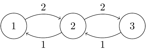
We can now determine the holding time distribution for each state.

State 1:
The total rate of leaving state 1 is $q_{1} = q_{12} + q_{13} = 2 + 0 = 2$ . This is also equal to $- q_{11}$ .
Therefore, the holding time in state 1, $T_{1}$ , is exponentially distributed with rate 2.
$T_{1} \sim Exp (2)$ .
The expected time spent in state 1 before a jump is $E [T_{1}] = 1/2$ .
State 2:
The total rate of leaving state 2 is $q_{2} = q_{21} + q_{23} = 1 + 2 = 3$ . This is equal to $- q_{22}$ .
Therefore, the holding time in state 2, $T_{2}$ , is exponentially distributed with rate 3.
$T_{2} \sim Exp (3)$ .
The expected time spent in state 2 before a jump is $E [T_{2}] = 1/3$ .
State 3:
The total rate of leaving state 3 is $q_{3} = q_{31} + q_{32} = 0 + 1 = 1$ . This is equal to $- q_{33}$ .
Therefore, the holding time in state 3, $T_{3}$ , is exponentially distributed with rate 1.
$T_{3} \sim Exp (1)$ .
The expected time spent in state 3 before a jump is $E [T_{3}] = 1$ .

This example is also worked through in the resource "Continuous time Markov jump processes", under Example 17.1.

Practice Problem

Now, let's solidify your understanding with a practice problem. The following resource presents the same rate diagram we just analyzed and asks you to determine the holding time parameters.

[PDF] MATH 447 - Worked Examples 7 - Continuous-Time Markov Chains

This document provides a worked example that directly tests the learning outcome of this lesson.

First, read Question 1, part a), found under the "Problems" heading on this page. Then, try to solve it yourself based on what we've just covered. Finally, check your work against the provided solution, which begins on the next page. The solution confirms that the holding time parameter for each state i is simply the sum of the rates of the arrows leaving that state.

Conclusion

In this lesson, we have connected the transition rates of a Markov process to the time it spends in each state. By leveraging the memoryless property, we established that holding times must be exponentially distributed.

Key Takeaways:

The time a continuous-time Markov process spends in a state $i$ , known as the holding time $T_{i}$ , is an exponentially distributed random variable.
The rate parameter of this exponential distribution, $q_{i}$ , is the sum of all transition rates leaving state $i$ : $q_{i} = \sum_{j \neq = i} q_{ij}$ .
This rate parameter can be found directly from the generator matrix $Q$ as the negative of the diagonal element for that state: $q_{i} = - q_{ii}$ .

So far, we have learned how to construct the generator matrix $Q$ and how to use it to find the holding time distributions. We now understand both where the process jumps to (probabilistically) and how long it waits before jumping. In our next lesson, we will combine these ideas to tackle a more complex question: how to calculate the probability of being in a certain state at a specific time $t$ in the future. This will lead us to a set of fundamental differential equations known as Kolmogorov's forward and backward equations.

Recommended resources