Compound Poisson Process Aggregates

Introduction

In our last session, we built the foundation for modeling aggregate claims by defining the compound Poisson process and deriving its key moments: the mean, variance, and moment generating function. We saw that $E [S (t)] = λ tE [X]$ and $Var [S (t)] = λ tE [X^{2}]$ . While these moments provide a high-level summary of the total claim amount, they don't tell the whole story. For an insurer to set premium rates, establish reserves, or design insurance products, it's essential to understand the full probability distribution of aggregate claims.

This lesson will equip you with the methods to calculate specific probabilities, such as the likelihood that total claims will exceed a certain threshold, and to compute conditional expectations. These skills are the bridge from theoretical process definition to practical actuarial problem-solving. We will explore both exact calculation methods and the powerful normal approximation, which becomes indispensable when dealing with large claim volumes.

Calculating Aggregate Claim Probabilities

Our goal is to find $P (S (t) \leq k)$ or $P (S (t) > k)$ . The method we use depends largely on the expected number of claims, $λ t$ .

1. The Exact Method (for small $λ t$ )

When the expected number of claims is small, we can calculate the probability of the aggregate claims $S (t)$ taking on a specific value $k$ by summing over all possible numbers of claims that could lead to that total. This is done by applying the law of total probability, conditioning on the number of claims $N (t)$ .

The probability mass function of $S (t)$ is given by:

P (S (t) = k) = n = 0 \sum \infty P (S (t) = k ∣ N (t) = n) \cdot P (N (t) = n)

Here:

$P (N (t) = n) = \frac{e ^{- λ t} ( λ t ) ^{n}}{n !}$ is the familiar Poisson probability.
$P (S (t) = k ∣ N (t) = n)$ is the probability that the sum of $n$ i.i.d. claim severity random variables equals $k$ . This is often denoted as $f_{X}^{* n} (k)$ , the $n$ -fold convolution of the severity distribution.

Calculating these convolutions can be intensive, but for simple discrete severities and a small number of claims, it is quite manageable. Let's examine a problem where this direct approach is used.

[PDF] Poisson Processes - Personal Homepages Server

This document contains a series of solved problems. We will focus on one that illustrates the exact calculation of an aggregate claim probability.

Please review Problem 5.20. The problem asks for the probability that aggregate losses exceed 3, where the expected number of claims is small (\lambda t = 1.25). Pay close attention to how the solution calculates the probabilities for S = 0, 1, 2, and 3. For each value of S, the author considers all possible numbers of claims (N) that could produce that total. For instance, to get S=3, you could have one claim of size 3, or two claims that sum to 3, or three claims that sum to 3. Each of these scenarios is a combination of a Poisson probability for the number of claims and a probability for the specific claim amounts.

This step-by-step calculation generates the probability mass function $p_{k} (t) = P (S (t) = k)$ . If we were to plot this PMF, we would see how the distribution of total claims evolves over time.

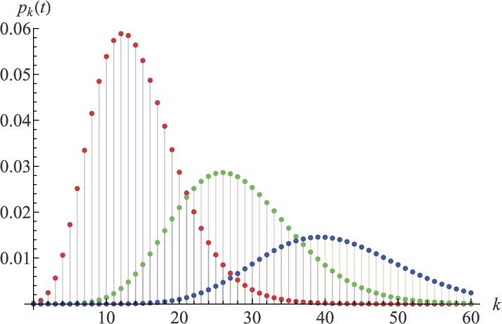
This graph illustrates the probability mass function, $p_k(t)$, of a compound Poisson process for three increasing values of time $t$. The red, green, and blue distributions correspond to small, medium, and large $t$, respectively. As $t$ increases, the mean of the distribution shifts to the right and the variance increases, causing the distribution to become more spread out and flatter. The exact method we just studied calculates the value of each individual point on these curves.

As you can see from the graph, as $t$ grows, the number of possible outcomes for $S (t)$ becomes very large, and the exact method quickly becomes computationally prohibitive. This is where approximations become essential.

2. The Normal Approximation (for large $λ t$ )

For a compound Poisson process where the expected number of claims $λ t$ is large, the distribution of the aggregate claims $S (t)$ can be approximated by a normal distribution. This is a direct consequence of a generalized Central Limit Theorem.

We can approximate $S (t)$ as:

S (t) \approx N (μ_{S}, σ_{S}^{2})

where the mean and variance are the ones we derived in the previous lesson:

$μ_{S} = E [S (t)] = λ tE [X]$
$σ_{S}^{2} = Var [S (t)] = λ tE [X^{2}]$

This allows us to answer probabilistic questions by standardizing the random variable and using standard normal tables. Let's see this powerful technique in action.

[PDF] Section 1: The Poisson Process - 1 ©ACTEX 2014

This ACTEX study manual provides an exam-focused example of using the normal approximation.

First, read the brief introduction to Compound Frequency Models. Then, study Example 2-1 in detail. This problem asks for the 90th percentile of the total number of claims over 13 weeks. Notice that the expected number of events (envelopes) is large: \lambda t = 50 \times 13 = 650. The solution proceeds by: Calculating the total \lambda t. Calculating the first and second moments of the severity distribution (number of claims per envelope). Applying the formulas for the mean and variance of the compound process. Using the standard normal distribution to find the desired percentile.

This approximation is a cornerstone of practical risk modeling, allowing actuaries to estimate probabilities for aggregate claims over long periods (e.g., a full year) where thousands of claims may occur.

Calculating Conditional Expectations

Beyond unconditional probabilities, actuaries often need to calculate expected values given some partial information. For example, what is the expected total claim amount, given that we know how many claims of a specific type occurred?

To solve such problems, we often use the decomposition property of Poisson processes. If a Poisson process with rate $λ$ has events that can be classified into $k$ independent types with probabilities $p_{1}, p_{2}, \dots, p_{k}$ , then the number of events of type $i$ , $N_{i} (t)$ , follows an independent Poisson process with rate $λ_{i} = λ p_{i}$ .

This is incredibly useful. Knowing the outcome of one process (e.g., the number of claims of type 2) gives us no information about the outcomes of the other independent processes.

Let's work through a classic problem that leverages this property.

This problem set from the ACTEX manual provides a perfect example of calculating a conditional expectation.

First, read Problem 1 from the problem set. It asks for the conditional expected value of coins found by Lucky Tom, given he found a specific number of 5-cent coins. Next, carefully study the provided solution. The key steps are: Decomposing the main Poisson process (rate \lambda=30 per hour) into three independent Poisson processes for coins of value 1, 5, and 10, with rates \lambda_1=18, \lambda_5=6, and \lambda_{10}=6. Recognizing that the total expected value is the sum of the expected values for each type. For the coins worth 5, the value is known to be 10 \times 5 = 50. This is the condition. Since the processes are independent, our knowledge about the 5-cent coins does not change our expectation for the 1-cent and 10-cent coins. Their expected values are simply their expected counts (\lambda_1 t and \lambda_{10} t) times their values.

The final expected value is calculated as:

E [Total Value ∣ N_{5} (1) = 10] = Expected value of 1s 1 \cdot E [N_{1} (1)] + Known value of 5s 5 \cdot 10 + Expected value of 10s 10 \cdot E [N_{10} (1)]

= 1 \cdot (λ_{1} \cdot 1) + 50 + 10 \cdot (λ_{10} \cdot 1) = 18 + 50 + 60 = 128

This demonstrates how the independence property simplifies conditional expectation problems significantly.

Conclusion

In this lesson, we have moved from the abstract moments of the compound Poisson process to concrete, calculable results. You have learned how to determine the probability of aggregate claims falling within a certain range and how to update expectations based on partial information.

Key Takeaways:

For a small expected number of claims ( $λ t$ ), aggregate claim probabilities can be calculated exactly by conditioning on the number of claims and summing the probabilities of all scenarios.
For a large expected number of claims, the distribution of aggregate claims $S (t)$ is well-approximated by a normal distribution with mean $λ tE [X]$ and variance $λ tE [X^{2}]$ .
Conditional expectations can often be simplified by decomposing a Poisson process into independent sub-processes for different event types. The expectation for the unconditioned event types remains unchanged.

This lesson concludes our first module on the applications of Markov and Poisson processes. We have built a solid foundation for modeling both the frequency and severity of events like insurance claims. In our next lesson, we will transition to continuous-time Markov jump processes, which will allow us to model movements between multiple states (e.g., healthy, sick, disabled, dead) where the time spent in each state is random.

Recommended resources