Breslow's Method for Baseline Survival Estimation

Introduction

In our last lesson, we focused on interpreting the output of a fitted Cox model, particularly the hazard ratios derived from the estimated coefficients $β^$ . We established that these hazard ratios are powerful tools for understanding the relative risk associated with different covariates. For instance, we can say that one group has 1.5 times the hazard of another. However, this leaves a critical question unanswered: what is the absolute probability that an individual will survive to a certain time?

To answer this, we need to estimate the one component of the Cox model that the partial likelihood method conveniently ignored: the baseline hazard function, $λ_{0} (t)$ , or its corresponding baseline survival function, $S_{0} (t)$ . This lesson will equip you with the primary non-parametric method for this task: Breslow's method. We will explore the formula, its intuition, and how it allows us to finally anchor our relative risk estimates to an absolute survival scale.

The Need for a Baseline

Recall the Cox model equation:

λ (t; Z) = λ_{0} (t) exp (β^{T} Z)

The corresponding survival function for an individual with covariates $Z$ is given by:

S (t; Z) = S_{0} (t)^{e x p (β^{T} Z)}

where $S_{0} (t) = exp (- \int_{0}^{t} λ_{0} (u) d u)$ is the baseline survival function. It's clear that without an estimate for $S_{0} (t)$ , we cannot compute absolute survival probabilities. The challenge is to estimate this function non-parametrically from the data, after having already estimated $β$ via partial likelihood.

Breslow's Estimator for the Cumulative Baseline Hazard

The most common approach is Breslow's method, which provides an estimate for the cumulative baseline hazard, $H^_{0} (t)$ . This is a direct analogue of the Nelson-Aalen estimator you encountered in Module 4, but it is adjusted to account for the covariate effects estimated by the Cox model.

The Breslow estimator is defined as a sum over the distinct event times $t_{i}$ up to time $t$ :

H^_{0} (t) = t_{i} \leq t \sum \frac{d _{i}}{\sum _{j \in R (t_{i})} exp ( β ^ ^{T} Z _{j} )}

Let's break down this formula:

$t_{i}$ : The $i$ -th distinct event time observed in the data.
$d_{i}$ : The number of events (e.g., deaths) occurring at time $t_{i}$ .
$R (t_{i})$ : The risk set at time $t_{i}$ , which includes all individuals who are still under observation and have not experienced the event just prior to time $t_{i}$ .
$β^$ : The vector of coefficients estimated from the Cox model.
$\sum_{j \in R (t_{i})} exp (β^^{T} Z_{j})$ : This is the denominator and the key component. For each individual $j$ in the risk set at time $t_{i}$ , we calculate their risk score, $exp (β^^{T} Z_{j})$ . The denominator is the sum of these risk scores over all individuals in the risk set. It represents the total "effective" risk at time $t_{i}$ , weighted by each individual's covariate profile.

The intuition is that the term for each event time, $\frac{d _{i}}{\sum e x p ( \dots )}$ , is an estimate of the discrete baseline hazard at that instant. By summing these up, we get the cumulative baseline hazard.

Once we have the cumulative baseline hazard, $H^_{0} (t)$ , we can easily estimate the baseline survival function using the standard relationship:

S^_{0} (t) = exp (- H^_{0} (t))

This yields a step function, similar to the Kaplan-Meier and Nelson-Aalen estimators, with jumps only at the observed event times.

The following reading provides a clear walk-through of this calculation.

Prediction Modeling with the Cox model - all about the baseline ...

This blog post by "Missing Data Solutions" provides an excellent, practical guide to calculating the baseline hazard. It demonstrates the Breslow estimator with clear R code.

Please read the following parts of the article: Start from the beginning to recap the model formula. Read the section "It all starts with the cumulative baseline hazard", which introduces the Breslow estimator. Finally, focus on the section "The Breslow estimator". Pay close attention to the formula and the R code that manually implements it. This will solidify your understanding of the mechanics.

A Practical Detail: Centering the Covariates

When we talk about a "baseline" hazard, we are referring to the hazard for a reference individual. By default, the Breslow formula above defines this reference person as someone with all covariate values equal to zero ( $Z = 0$ ). This might not always be a meaningful reference (e.g., if a covariate is age, a baseline of age=0 may be irrelevant).

A more common approach is to define the baseline relative to an "average" person, where the covariates are set to their sample mean values, $Z ˉ$ . This is known as centering.

When centering is applied, the Breslow estimator formula is slightly modified:

H^_{0} (t) = t_{i} \leq t \sum \frac{d _{i}}{\sum _{j \in R (t_{i})} exp ( β ^ ^{T} ( Z _{j} - Z ˉ ) )}

This adjustment ensures that $S^_{0} (t)$ represents the survival function for an individual with the average covariate profile of the study population. In most software, including R's survival package, this is the default behavior.

The following reading explains this concept of centering very clearly.

Prediction Modeling with the Cox model - all about the baseline ...

Let's return to the same article to understand the practical implications of centering.

Please read the section "What is the difference..." and continue through the worked example of mean centering. This will show you how the choice of baseline (all-zero vs. average covariates) changes the calculation and the resulting cumulative hazard values.

Implementation in R

In practice, you will rarely need to calculate the Breslow estimate by hand. The R survival package provides functions to do this automatically from a fitted coxph object.

The primary functions are basehaz() and survfit().

basehaz(fit) directly computes the cumulative baseline hazard. The argument centered=TRUE (the default) or centered=FALSE controls the centering behavior we just discussed.
survfit(fit) is a more general function that can compute survival curves. When applied to a coxph object, it estimates the survival function for a reference individual. By default, this is the "average" individual (equivalent to basehaz with centered=TRUE).

The following reading provides a concise overview of using survfit for this purpose.

[PDF] Tied survival times; estimation of survival probabilities - MyWeb

These lecture notes from the University of Iowa provide a more formal statistical perspective and introduce the survfit function.

Please read the subsection on using survfit.coxph. Note how it connects the output of coxph to the estimation of the baseline survival curve and confirms that the default is a centered model.

Visualizing the Result

The result of this process is an estimated step function for baseline survival, $S^_{0} (t)$ . In the next lesson, we will see how to combine this with our estimated coefficients to generate survival curves for any individual.

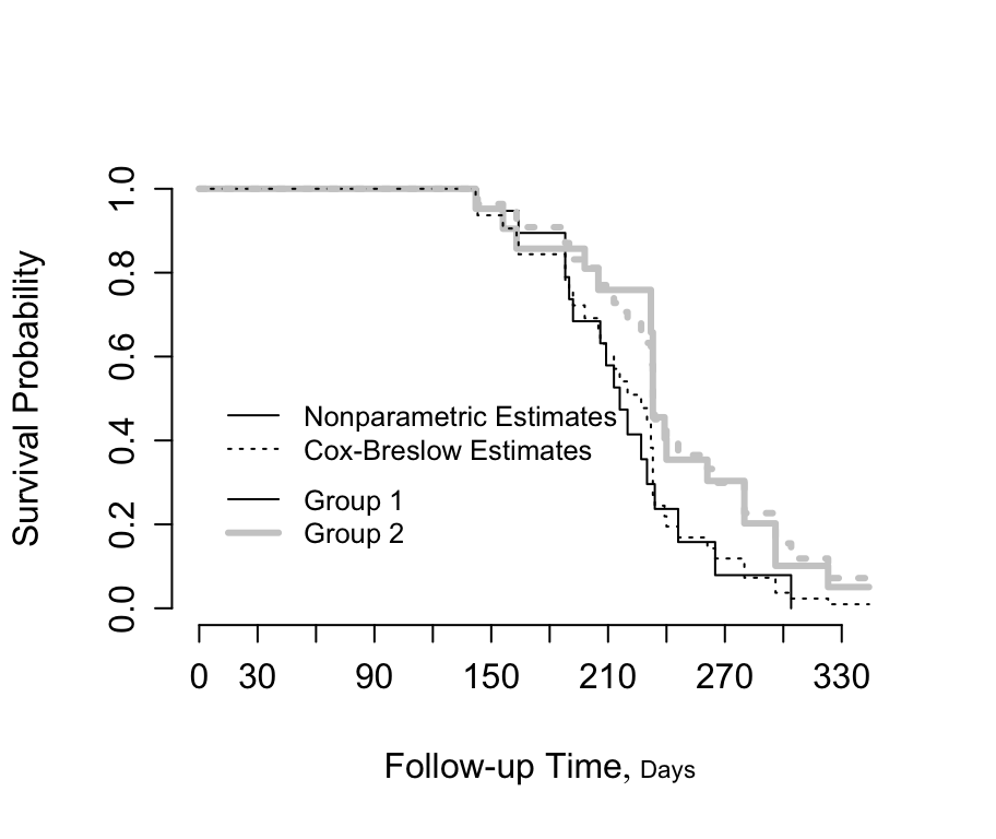
The plot below gives a preview of this. The "Nonparametric Estimates" (solid lines) are likely separate Kaplan-Meier curves for two groups, which make no modeling assumptions. The "Cox-Breslow Estimates" (dotted lines) are the survival curves for the same two groups, but generated from a single Cox model. They are derived by applying the group-specific hazard ratio to a common estimated baseline survival function found using Breslow's method. Notice how the model-based curves are smoother versions of the empirical KM curves, reflecting the smoothing effect of the proportional hazards assumption.

This plot compares survival curves estimated directly from the data for two groups (Nonparametric Estimates, likely Kaplan-Meier) with those estimated from a Cox model using the Breslow estimator to find the baseline survival (Cox-Breslow Estimates).

Conclusion

In this lesson, we have filled the main gap in our ability to use the Cox model for prediction. While partial likelihood gave us the relative effects of covariates ( $β^$ ), Breslow's method provides the missing piece: a non-parametric estimate of the baseline survival function, $S^_{0} (t)$ .

Key Takeaways:

The Cox model requires an estimate of the baseline survival function, $S_{0} (t)$ , to calculate absolute survival probabilities.
Breslow's method is the standard non-parametric technique for estimating the cumulative baseline hazard, $H^_{0} (t)$ .
The Breslow estimator is analogous to the Nelson-Aalen estimator but weights the risk set by the covariate-derived risk scores from the Cox model.
The baseline can be defined for a reference individual with zero covariates (centered=FALSE) or for an individual with average covariates (centered=TRUE), which is the common default.
The estimated baseline survival function is calculated as $S^_{0} (t) = exp (- H^_{0} (t))$ .

Now that we can estimate both $β^$ and $S^_{0} (t)$ , we have all the necessary components for prediction. In our next lesson, we will put them together to predict survival probabilities and plot survival curves for individuals with specific covariate values.

Recommended resources