Predicting Survival Probabilities with Cox Models

Introduction

In our previous lesson, we addressed a crucial step in making the Cox model practical for prediction: estimating the baseline survival function, $S_{0} (t)$ , using Breslow's method. You'll recall that by itself, the Cox model only provides relative risk through hazard ratios, $exp (β^{T} Z)$ . By estimating $S_{0} (t)$ , we established an anchor for these relative risks.

This lesson is where we put all the pieces together. We will combine the estimated coefficients, $β^$ , with the estimated baseline survival function, $S^_{0} (t)$ , to achieve our ultimate goal: predicting absolute survival probabilities and generating complete survival curves for individuals with specific characteristics. This allows us to move from statements like "smokers have twice the hazard" to "a 60-year-old smoker has a 75% probability of surviving the next five years."

The Prediction Formula

The power of the Cox model lies in its ability to relate an individual's survival function, $S (t; Z)$ , to the baseline survival function, $S_{0} (t)$ . As we saw previously, the relationship is:

S (t; Z) = S_{0} (t)^{e x p (β^{T} Z)}

Once we have fit our model, we have estimates for both $β$ and $S_{0} (t)$ . Therefore, to predict the survival probability at time $t$ for a new individual with a specific vector of covariate values, $Z_{new}$ , we simply plug our estimates into the formula:

S^(t; Z_{new}) = S^_{0} (t)^{e x p (β^^{T} Z_{new})}

Here, $exp (β^^{T} Z_{new})$ is the estimated hazard ratio for our new individual relative to the baseline. The formula elegantly shows that we are taking the baseline survival curve, $S^_{0} (t)$ , and raising it to the power of the individual's hazard ratio.

If the hazard ratio is greater than 1 (higher risk), the survival curve will be pushed down, resulting in lower survival probabilities.
If the hazard ratio is less than 1 (lower risk), the survival curve will be pulled up, resulting in higher survival probabilities.

The following resource provides a formal statement of this fundamental prediction formula.

[PDF] The Cox Hazard Model for Claims Data | Variance

This paper from the Casualty Actuarial Society provides a clear, applied view of the Cox model in an insurance context.

Please read the section that introduces the formula for the estimated survival probability. You will find it right after the formula for the hazard ratio (HR). Focus on the equation for Si(t). This is the mathematical foundation for everything we will do in this lesson.

A Note on Centering

Remember from our last lesson that the baseline survival function $S^_{0} (t)$ is typically estimated for a reference individual whose covariates are at the sample mean, $Z ˉ$ . When this is the case, the term in the exponent needs to be adjusted to reflect the hazard ratio relative to this average person. The prediction formula becomes:

S^(t; Z_{new}) = S^_{0} (t)^{e x p (β^^{T} (Z_{new} - Z ˉ))}

Fortunately, most statistical software, including R, handles this centering automatically, but it's crucial to be aware of what is happening under the hood to ensure correct interpretation.

Prediction in Practice with R

While the formula provides the theory, in practice we rely on functions to perform these calculations. In R, the primary function for this is predict(), applied to a coxph object. A related, and often more convenient, function is survfit().

To generate predictions for a new individual, we supply their covariate values in a data.frame to the newdata argument of these functions. The predict() function is particularly instructive as it can return the component parts of the prediction.

The following reading walks through the different prediction types available in R's predict.coxph function, culminating in the survival probability.

Prediction Modeling with the Cox model - all about the baseline ...

We return to this practical blog post to see how predictions are generated in R.

Please read the following sections to understand the building blocks of prediction: Start with the subsection on the predict.coxph function. Read about type="lp" and type="risk". This shows how R calculates the linear predictor (\hat{\boldsymbol{\beta}}^T (\boldsymbol{Z} - \bar{\boldsymbol{Z}})) and the hazard ratio (\exp(\text{lp})). Read about type="expected". This gives the individual's cumulative hazard, H(t; \boldsymbol{Z}) = H_0(t) \times \text{risk}. Finally, focus on type="survival". You will see that the survival probability is simply calculated as \exp(-\text{expected}), which directly corresponds to our formula S(t) = \exp(-H(t)). Notice how the code demonstrates this relationship clearly.

The survfit(cox_model, newdata = ...) function is often a more direct way to get what we want: a full survival curve for a new observation, which can then be easily plotted or queried for specific probabilities.

Visualizing Individual Survival Curves

The real power of prediction is not just calculating a single probability, but generating an entire survival curve tailored to an individual. By applying the prediction formula at all event times, we can plot $S^(t; Z_{new})$ as a function of $t$ . This provides a complete picture of an individual's expected survival trajectory based on the model.

The image below shows the output of such a process. It displays the predicted survival curves for five different individuals, each with a distinct risk score derived from their covariates.

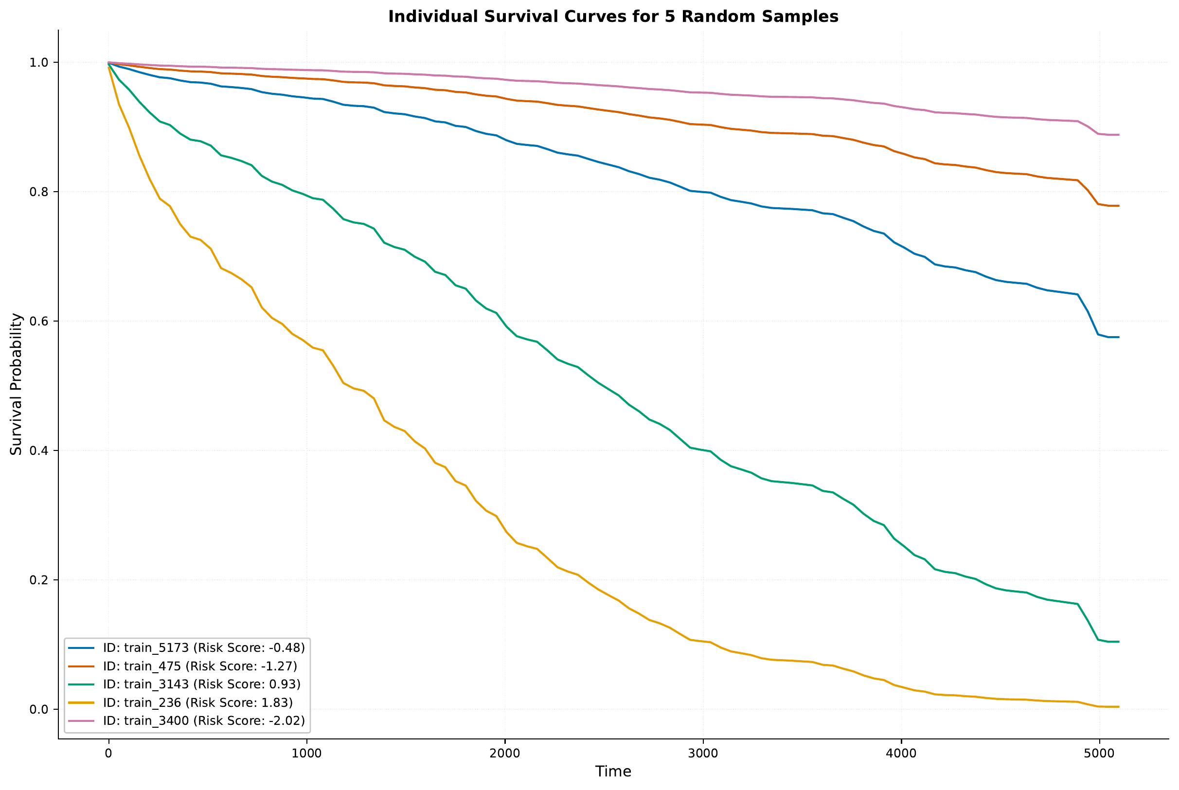
These are predicted survival curves for five individuals from a dataset. Each curve corresponds to a specific set of covariate values, summarized by a single "Risk Score" (the linear predictor). Notice how individuals with higher (positive) risk scores have steeper curves, indicating a lower survival probability over time, while those with lower (negative) risk scores have flatter curves and better survival prospects.

We can also use this technique to compare the expected survival of different, well-defined groups. For example, we can generate and plot the predicted survival curves for "male, treatment group" vs. "male, placebo group".

This plot shows predicted survival curves from a Cox model for four distinct groups based on sex and treatment status. This is a common and powerful way to visualize the model's predictions and the interactive effect of different covariates.

An Applied Example: Predicting Insurance Claim Times

Let's now turn to a detailed example from the actuarial field. The following reading uses a Cox model to analyze the time until a workers' compensation claim occurs, using industry and season as covariates. It perfectly demonstrates how to interpret predicted survival curves for different groups and scenarios.

[PDF] The Cox Hazard Model for Claims Data | Variance

Let's continue with the actuarial paper. We will now look at how the authors use their fitted model to make and interpret predictions.

Please read the following parts of Section 9, "Interpretation of results": Start with the paragraph that begins "For the purposes of comparing...". Study Figure 3 and the accompanying text. This shows the baseline prediction: comparing industries without considering time-varying effects. Note how they interpret the probabilities (e.g., "there is a 58% chance that there will be no claims before the 100th day"). Next, read about the introduction of a time-dependent covariate, SEASON_EVENT, starting from the paragraph "Estimation of survival...". Finally, carefully study the two examples that follow. The first analyzes a policy starting on April 1st (see Figure 5), and the second analyzes a policy starting on August 1st (see Figure 7). Observe how the predicted survival functions change dramatically depending on when the policy starts, as this affects when the "winter season" risk factor is active. This is an excellent, practical demonstration of prediction with time-varying covariates.

This example highlights how a fitted Cox model can be used to generate nuanced, context-specific predictions that are invaluable for risk assessment in insurance and beyond.

Conclusion

In this lesson, we have completed the journey from fitting a Cox model to using it for prediction. By combining the estimated baseline survival function with the estimated coefficients, we can now generate survival probabilities and full survival curves for any individual, given their covariate values.

Key Takeaways:

The core prediction formula is $S^(t; Z_{new}) = S^_{0} (t)^{e x p (β^^{T} Z_{new})}$ .
This formula effectively adjusts the baseline survival curve based on an individual's specific hazard ratio.
In R, the predict() and survfit() functions, using the newdata argument, are the practical tools for generating these predictions.
The output can be visualized as individual survival curves, which provide a powerful way to compare risk profiles and understand the impact of covariates.

We now have a complete toolkit for fitting and interpreting the Cox model. However, all our work rests on the crucial assumption of proportional hazards. In our next lesson, we will learn how to formally test this assumption to ensure that our model is appropriate for the data and that our predictions are reliable.

Recommended resources