Understanding Hazard Ratios and Confidence Intervals in Cox Models

From Coefficients to Hazard Ratios

Recall the fundamental equation of the Cox model for an individual with covariates $Z=(Z_1,...,Z_p)$:

The estimated coefficient, ${\hat{\beta }}_k$, quantifies the change in the logarithm of the hazard for a one-unit increase in the corresponding covariate $Z_k$, assuming all other covariates are held constant. While mathematically correct, interpreting log-hazards is not intuitive.

To make the interpretation more direct, we exponentiate the coefficient to obtain the Hazard Ratio (HR):

The hazard ratio is a multiplicative factor. It tells us how the hazard rate is multiplied for every one-unit increase in the covariate $Z_k$.

The following video provides an excellent explanation of the relationship between coefficients and hazard ratios, and how to interpret them.

As the video explains, the interpretation of a hazard ratio is straightforward:

• $HR>1$ (or $\beta >0$): An increase in the covariate is associated with an increased hazard (higher risk). For example, an HR of 1.5 means a 50% increase in the hazard.
• $HR<1$ (or $\beta <0$): An increase in the covariate is associated with a decreased hazard (a protective effect). For example, an HR of 0.7 means a 30% reduction in the hazard.
• $HR=1$ (or $\beta =0$): The covariate has no effect on the hazard.

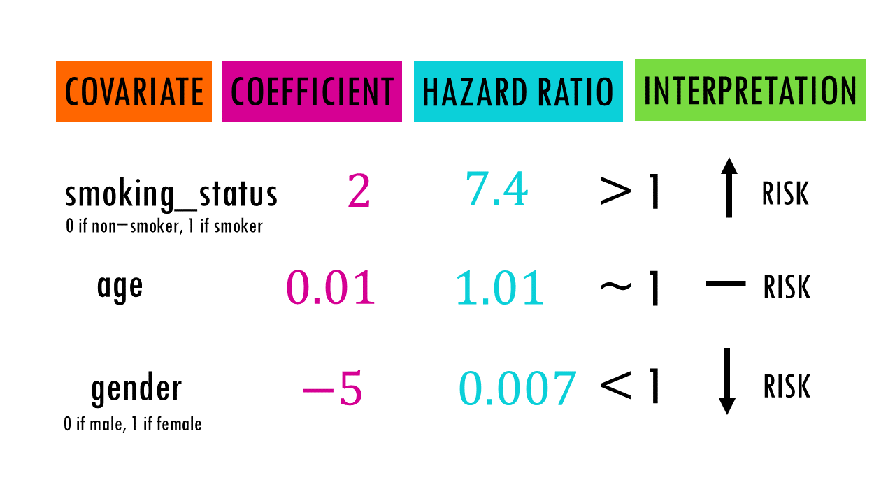
This relationship is summarized in the diagram below.

A Framework for Interpretation

To solidify your understanding, we will work through a structured guide on interpreting a typical Cox regression output table. This involves looking not just at the hazard ratio, but also its confidence interval and p-value.

As the reading highlights, the interpretation depends on the type of covariate:

• For a binary covariate (e.g., smoking_status coded as 0 for non-smoker, 1 for smoker), the HR compares the hazard of the group coded '1' to the hazard of the group coded '0'. An HR of 7.4, as in the diagram above, would mean smokers have 7.4 times the hazard of non-smokers.
• For a continuous covariate (e.g., age in years), the HR represents the change in hazard for each one-unit increase. An HR of 1.02 for age means the hazard increases by 2% for each additional year of age. Note that for a ten-year increase, the effect is compounded: $1.02^{10}\approx 1.22$, representing a 22% increase in hazard.

Assessing Statistical Significance with Confidence Intervals

The estimated coefficient $\hat{\beta }$ is a point estimate; it has uncertainty. In the previous lesson, you learned that the Newton-Raphson algorithm used to maximize the partial likelihood also yields an estimate of the variance-covariance matrix of the coefficients. From this, we can obtain the standard error, $SE({\hat{\beta }}_k)$, for each coefficient.

Given your statistics background, you'll know we can construct a 95% confidence interval for the true coefficient ${\beta }_k$ as:

To get the 95% confidence interval for the hazard ratio, we simply exponentiate the endpoints of the interval for the coefficient:

This confidence interval is fundamental for interpretation. If the confidence interval for the hazard ratio contains the value 1.0, the effect of the covariate is not statistically significant at the 5% level. This is because a hazard ratio of 1.0 implies no effect, and the interval suggests that "no effect" is a plausible value for the true, unknown hazard ratio. This is equivalent to having a p-value greater than 0.05.

The following video segment revisits this crucial point.

Practice: Interpreting a Model Output

Let's apply these concepts to a typical model output. The table below shows the results from a Cox regression model analyzing factors associated with patient mortality in a clinical trial.

Let's interpret the results for three key variables from this table: ejection_fraction, serum_creatinine, and high_blood_pressure.

1. Ejection Fraction (a measure of heart function; continuous variable)

   • Coefficient ($\hat{\beta }$): -0.05
   • Hazard Ratio (HR): 0.95
   • Interpretation: For each one-unit percentage point increase in ejection fraction, the hazard of death is multiplied by 0.95. This means the risk of death decreases by 5% ($1-0.95=0.05$).
   • Significance: The p-value is <0.005, which is highly significant. The 95% CI for the HR is [0.93, 0.97] (calculated from the coef and se(coef)), which does not contain 1.0. This confirms the strong statistical significance of this protective factor.

2. Serum Creatinine (a measure of kidney function; continuous variable)

   • Coefficient ($\hat{\beta }$): 0.32
   • Hazard Ratio (HR): 1.38
   • Interpretation: For each 1 mg/dL increase in serum creatinine, the hazard of death increases by 38%.
   • Significance: The p-value is <0.005, indicating a highly significant effect. The 95% CI for the HR is [1.20, 1.58], which is well above 1.0, reinforcing that higher creatinine is a significant risk factor.

3. High Blood Pressure (binary variable, likely 0=No, 1=Yes)

   • Coefficient ($\hat{\beta }$): 0.48
   • Hazard Ratio (HR): 1.61
   • Interpretation: Patients with high blood pressure have a 61% higher hazard of death compared to those without high blood pressure, holding other factors constant.
   • Significance: The p-value is 0.03, which is less than 0.05. The 95% CI for the HR is [1.05, 2.46]. Since this interval is entirely above 1.0 (though the lower bound is close), we conclude the effect is statistically significant at the 5% level.

Conclusion

In this lesson, we have bridged the gap between estimating Cox model parameters and extracting actionable insights from them. You are now equipped to interpret the standard output of a Cox regression analysis, a core competency in survival modeling.

Key Takeaways:

• The hazard ratio (HR), calculated as $\exp (\hat{\beta })$, provides an intuitive, multiplicative measure of a covariate's effect on risk.
• An HR greater than 1 indicates increased risk, while an HR less than 1 indicates a protective effect.
• The interpretation of the HR depends on whether the covariate is continuous, binary, or categorical.
• The 95% confidence interval for the HR is crucial for assessing statistical significance. If the interval contains 1.0, the result is not statistically significant at the 5% level.
• P-values provide a complementary check for significance, with $p<0.05$ typically indicating a significant result.

We have successfully modeled the relative risk associated with different covariates. However, the Cox model's partial likelihood approach leaves the baseline hazard ${\lambda }_0(t)$ unspecified. In our next lesson, we will address this by learning how to estimate the baseline survival function, ${\hat{S}}_0(t)$, using Breslow's method. This will allow us to move from relative risk to calculating absolute survival probabilities for individuals with specific characteristics.