Mixed-Precision Training: Accelerating Training and Reducing Memory

Part 1: The Core Idea of Mixed-Precision Training

At its heart, mixed-precision training is a simple but powerful idea: instead of performing all calculations using the standard 32-bit floating-point format (FP32), we strategically use a combination of lower-precision 16-bit formats (like FP16 or BF16) for the bulk of the work and reserve the high-precision FP32 format for operations that require it.

This hybrid approach delivers two transformative benefits:

1. Reduced Memory Usage: A 16-bit number occupies half the memory of a 32-bit number. By using 16-bit formats for model weights, gradients, and activations, you can nearly halve the VRAM required. This allows you to train larger models, use larger batch sizes, or simply fit the training process onto less expensive hardware.
2. Faster Computation: Modern GPUs, particularly those with NVIDIA's Tensor Cores, are specifically designed to perform mathematical operations on 16-bit numbers at a much higher rate than on 32-bit numbers—often achieving speedups of 2x or more on matrix multiplications and convolutions, which are the computational core of transformer models.

To get a solid grasp of these concepts, let's start with a foundational reading.

Part 2: A Tale of Two Halves: FP16 vs. BF16

To understand mixed-precision training deeply, we need to look at the data types themselves. A floating-point number is typically composed of three parts: a sign bit, an exponent (which determines the range of numbers you can represent), and a mantissa or fraction (which determines the precision, or the number of significant digits).

The two main 16-bit formats, FP16 and BF16, make different trade-offs in how they allocate their 16 bits.

• FP16 (Half-Precision):

  • Structure: 1 sign bit, 5 exponent bits, 10 mantissa bits.
  • Characteristics: The 10-bit mantissa provides relatively good precision for a 16-bit float. However, the 5-bit exponent gives it a very limited dynamic range. It cannot represent extremely large or extremely small numbers, making it prone to "overflow" (becoming infinity) or "underflow" (becoming zero).

• BF16 (Brain Floating-Point):

  • Structure: 1 sign bit, 8 exponent bits, 7 mantissa bits.
  • Characteristics: The 8-bit exponent is the same as in FP32, giving BF16 the same dynamic range as FP32. This makes it far more resilient to overflow and underflow. The trade-off is a smaller 7-bit mantissa, meaning it has lower precision than FP16.

For LLM training, the large dynamic range of BF16 has proven to be a significant advantage. The training process involves a wide range of numerical values, and BF16's ability to handle them without underflow often makes it a more stable and easier-to-use choice than FP16, especially on hardware that supports it natively (like NVIDIA A100/H100 GPUs and Google TPUs).

The following video from NVIDIA provides a clear explanation of these floating-point representations and their implications.

Part 3: The Stability Challenge and Its Solutions

The benefits of 16-bit computation are clear, but why can't we just switch everything to FP16 or BF16 and call it a day? The answer lies in numerical stability. As hinted at, lower precision introduces two major risks.

Problem 1: Gradient Underflow

During backpropagation, especially in deep networks and late in training, gradients can become extremely small. The limited range of FP16 means these tiny, but still important, gradient values can be rounded to zero (underflow). When this happens, the model stops learning from that part of the data.

• Solution: Loss Scaling
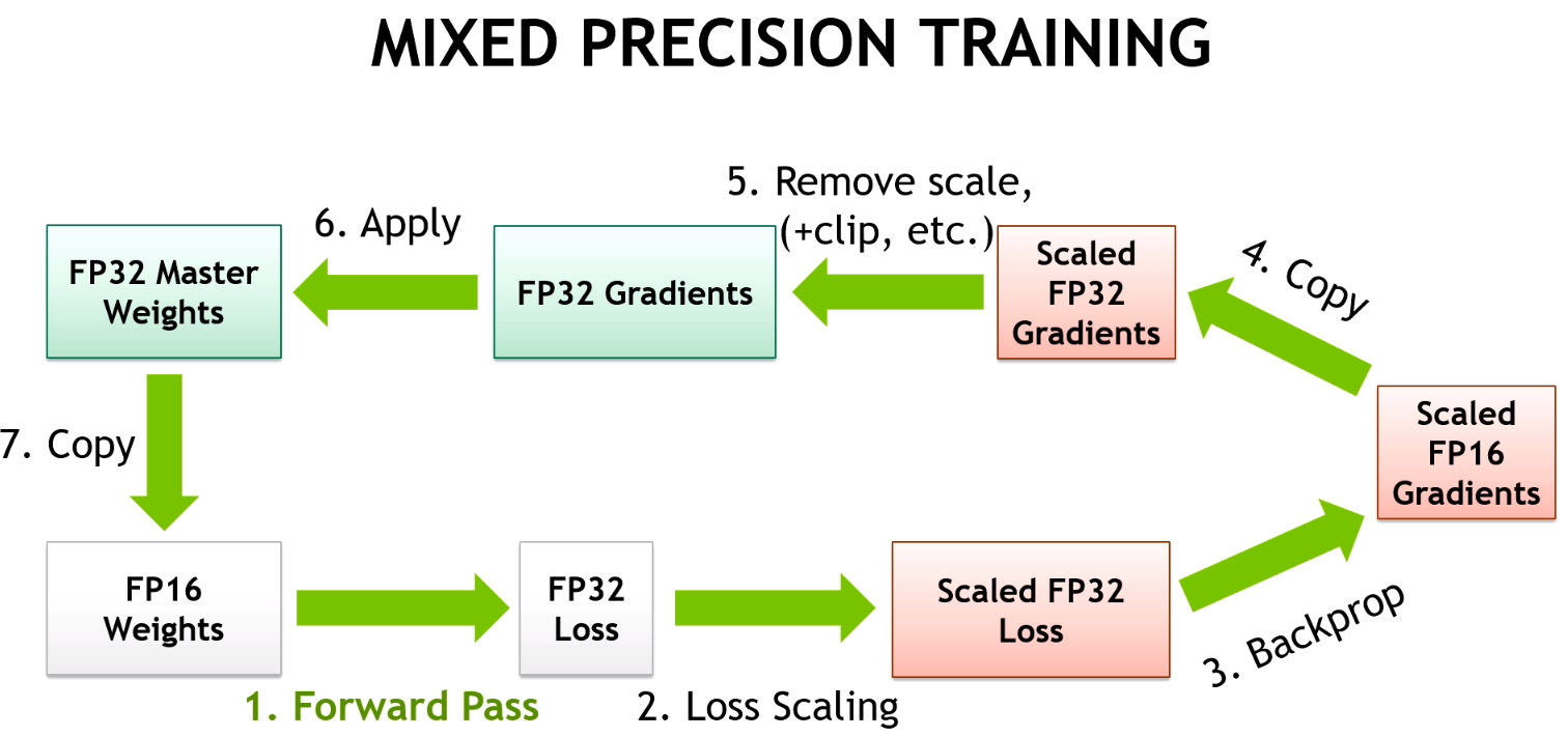
  The ingenious solution is to scale up the loss value by a large factor (e.g., 2^16) right before starting the backward pass. Due to the chain rule of calculus, this scales up all the gradients by the same factor, effectively "shifting" them into the representable range of FP16 and preventing underflow. Before the optimizer updates the weights, these gradients are scaled back down to their original values.

Problem 2: Precision Loss in Weight Updates

Even if gradients are preserved, another problem arises. The weight update is typically a small value (gradient multiplied by a small learning rate). When you add this tiny update to a large weight value in a low-precision format like FP16, the update can be lost due to rounding errors. For example, 1.0000 + 0.0001 might just get rounded back to 1.0000.

• Solution: FP32 Master Weights
  To solve this, a master copy of the model's weights is maintained in the full FP32 format. The forward and backward passes use a temporary FP16 copy for speed and memory savings. However, the final update step—where the scaled-down gradients are applied—is performed on the high-precision FP32 master weights. A new FP16 copy is then created for the next iteration.

This entire process is visualized perfectly in the following flowchart.

To see a detailed explanation of these problems and solutions, let's return to the NVIDIA video.

Part 4: Automatic Mixed Precision in PyTorch

Given your background in PyTorch, it's valuable to see how these complex steps are made simple in practice. You don't need to manually manage master weights or loss scaling. PyTorch provides a built-in library called Automatic Mixed Precision (AMP) that handles it all for you with just a few lines of code.

There are two main components:

1. torch.cuda.amp.autocast(): A context manager that you wrap around your model's forward pass. It automatically chooses the optimal precision for each operation—running operations like matrix multiplies in FP16/BF16 and keeping sensitive operations like normalizations in FP32.
2. torch.cuda.amp.GradScaler(): An object that automates loss scaling. You use it to wrap your loss and backward pass, and it dynamically adjusts the scaling factor to prevent underflow without causing overflow.

This final clip from the NVIDIA webinar shows exactly how to integrate AMP into a standard PyTorch training loop.

Conclusion

Today, we've moved from the abstract world of FLOPs to the practical realities of GPU hardware. You've learned that mixed-precision training isn't just a minor tweak; it's a fundamental enabling technology for training large language models. By intelligently combining 16-bit and 32-bit formats, we can achieve significant speedups and memory savings while preserving the numerical stability required for convergence.

Key Takeaways:

• Dual Benefits: Mixed-precision training accelerates computation by leveraging specialized hardware (Tensor Cores) and reduces memory footprint by up to 50%.
• FP16 vs. BF16: FP16 offers higher precision but a limited numerical range, risking underflow. BF16 has a massive range (same as FP32) but lower precision, making it more stable and often preferred for modern LLM training.
• Stability Mechanisms: To counter the risks of low precision, two key techniques are used: loss scaling to prevent gradient underflow and FP32 master weights to ensure accurate weight updates.
• Automated Implementation: Frameworks like PyTorch provide Automatic Mixed Precision (AMP) libraries that handle these complex mechanics automatically, making it easy to gain the benefits in your own training scripts.

What's Next?

We've now covered how to estimate the compute for a training run and how to make that run more efficient on a single GPU. The next logical step is to scale beyond the limits of a single machine. How do you train a model that is too large to fit in one GPU's memory, or how do you use hundreds of GPUs to finish training in weeks instead of years?

In our next lesson, we will explore the essential distributed training paradigms for LLMs, including Data Parallelism, Tensor Parallelism, and Pipeline Parallelism.