Gradient Accumulation for Larger Batches

1. The Core Idea: Simulating Large Batches

The fundamental trade-off in training deep neural networks is between batch size and memory.

• Large Batch Sizes are Good: They provide a more accurate estimate of the gradient across the entire dataset, leading to more stable training updates and often allowing for higher learning rates.
• Large Batch Sizes are Expensive: Each sample in a batch requires its own set of intermediate activations to be stored in GPU VRAM for the backward pass. For a large model like a transformer and a long sequence length, the memory required for even a moderate batch size can easily exceed what's available on a single GPU.

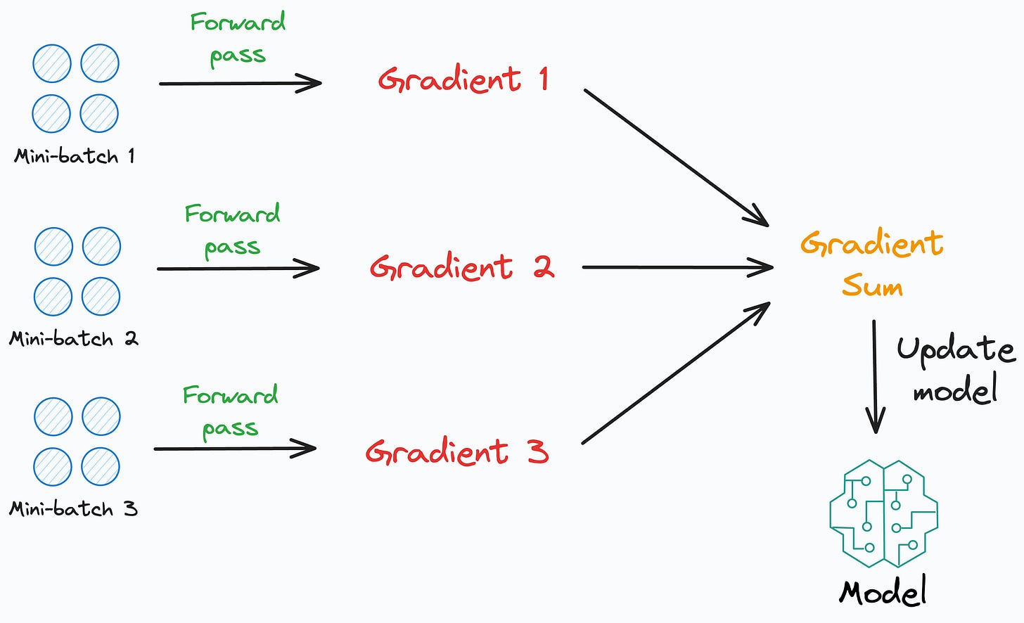
Gradient accumulation elegantly sidesteps this issue. Instead of processing a single large batch, we break it down into several smaller micro-batches that do fit in memory. We then process each micro-batch sequentially, calculate its gradients, and add them up. Only after processing all the micro-batches do we update the model's weights using the accumulated gradient.

The image below illustrates this process perfectly.

2. The Mechanics of Gradient Accumulation

To understand how this works in practice, let's break down the steps and contrast them with a standard training loop.

Standard Training Loop (for one batch):

1. optimizer.zero_grad(): Clear any gradients from the previous step.
2. outputs = model(inputs): Forward pass to get model predictions.
3. loss = criterion(outputs, labels): Calculate the loss.
4. loss.backward(): Compute gradients for all model parameters.
5. optimizer.step(): Update the model's weights using the computed gradients.

Gradient Accumulation Loop (simulating one large batch):
Let's say we want an effective batch size of 128, but can only fit a micro-batch of 32 samples in memory. This means we need 128 / 32 = 4 accumulation steps.

The process is as follows:

1. optimizer.zero_grad(): Clear gradients at the very beginning.
2. For accumulation_steps (e.g., 4 times):
   a. Fetch a micro-batch of data (size 32).
   b. outputs = model(inputs): Forward pass.
   c. loss = criterion(outputs, labels): Calculate loss for the micro-batch.
   d. Important: If your loss function is an average (like most are), you need to normalize it: loss = loss / accumulation_steps. This ensures that each micro-batch contributes its proportional share to the total loss.
   e. loss.backward(): Compute gradients and add them to the existing gradients. PyTorch does this by default when you call .backward() multiple times without zero_grad().
3. After the loop finishes:
   a. optimizer.step(): Update the weights using the summed gradients from all 4 micro-batches.
   b. Now that the update is done, the accumulated gradients are no longer needed for the next large batch, so we would call optimizer.zero_grad() before the next accumulation cycle begins.

To formalize this, please read the following brief document, which covers the motivation, concept, and mathematical formulation.

3. Implementation in PyTorch

Given your experience with PyTorch, you'll find the implementation remarkably straightforward. It primarily involves adding a simple conditional statement to your training loop to control when optimizer.step() and optimizer.zero_grad() are called.

The following resource provides an exceptionally clear guide with code examples, progressing from a basic implementation to more advanced use cases relevant to your goals, such as with transformer models.

Here's a condensed example synthesizing the logic from the resources. Notice how the update step is guarded by the if condition.

# Hyperparameters
effective_batch_size = 256
micro_batch_size = 32
accumulation_steps = effective_batch_size // micro_batch_size # This would be 8

model = ...
optimizer = ...
dataloader = ... # with batch_size = micro_batch_size

model.train()
optimizer.zero_grad() # Clear gradients at the start of the epoch

for i, (inputs, labels) in enumerate(dataloader):
    # Forward pass
    outputs = model(inputs)
    loss = criterion(outputs, labels)

    # Normalize loss to account for accumulation
    loss = loss / accumulation_steps
    
    # Backward pass to accumulate gradients
    loss.backward()

    # Perform weight update after `accumulation_steps`
    if (i + 1) % accumulation_steps == 0:
        optimizer.step()       # Update weights
        optimizer.zero_grad()  # Clear gradients for the next accumulation cycle

4. Advantages and Caveats

While powerful, gradient accumulation is not a free lunch. It's essential to understand its trade-offs.

Advantages:

• Enables Large Batch Training: Its primary benefit is allowing you to train with large effective batch sizes that would otherwise be impossible due to memory constraints.
• Improves Training Stability: The resulting gradient from a larger effective batch is a better approximation of the true gradient, which can lead to a more stable training process.
• Simple to Implement: As you've seen, it requires minimal changes to a standard training loop.

Challenges and Caveats:

• Increased Training Time: You are trading memory for computation. To achieve one weight update, you must perform multiple forward and backward passes. This increases the total wall-clock time for training.
• Optimizer and Layer Dynamics: Some parts of a model might behave differently. For example, if you use Batch Normalization, its statistics will be calculated on the small micro-batches, not the large effective batch. This means the training dynamics are not identical to true large-batch training. This is less of a concern for modern LLMs that primarily use Layer Normalization, which is independent of the batch size.
• Synchronization Overhead: In a distributed setting (which we will cover next), accumulating gradients requires careful synchronization across devices, which can add complexity.

Conclusion

Today, you've added another crucial technique to your arsenal for training large-scale models. Gradient accumulation is a simple yet powerful method to overcome hardware memory limitations by simulating large batch sizes. By breaking down large batches into smaller micro-batches and summing their gradients before a weight update, you can achieve the stability benefits of large-batch training without needing a proportionally large GPU.

Key Takeaways:

• Core Concept: Gradient accumulation trades compute time for memory savings by performing multiple forward/backward passes for a single optimizer step.
• Implementation: The logic involves calling loss.backward() in a loop and only calling optimizer.step() and optimizer.zero_grad() after a set number of accumulation steps.
• Loss Normalization: Remember to divide your loss by the number of accumulation steps to ensure the final accumulated gradient has the correct magnitude.
• Trade-offs: The main drawback is increased training time. It's also important to be aware of how it might interact with certain layers like Batch Normalization.

What's Next?

We've now explored two key strategies for optimizing training on a single GPU: mixed precision and gradient accumulation. However, to train state-of-the-art LLMs, we must go beyond a single device. How do we train a model that is too large to fit in one GPU's memory, or how do we use hundreds of GPUs to finish training in weeks instead of years?

In our next lesson, we will dive into the distributed training paradigms for LLMs: Data Parallelism, Tensor Parallelism, and Pipeline Parallelism, which are the keys to unlocking true large-scale training.