Introduction
Welcome to our next lesson on scaling LLMs. In our previous lessons, we mastered techniques like mixed-precision training and gradient accumulation to maximize the efficiency of a single GPU. These are powerful tools, but they have their limits. The sheer size of state-of-the-art models (hundreds of billions of parameters) and the massive datasets they are trained on mean that a single GPU is often not enough, either because the model won't fit in memory or because training would take an impractically long time.
To overcome these barriers, we must move from a single GPU to a distributed cluster of many GPUs working in concert. This lesson unpacks the three fundamental paradigms for distributed training: Data Parallelism, Tensor Parallelism, and Pipeline Parallelism. Understanding these strategies is crucial for comprehending how today's largest models are built and for designing your own scalable training systems.
1. The Core Challenge: Splitting the Work
When you have multiple GPUs, the core question is: how do you divide the work? There are two main things you can split: the data or the model. This choice leads to our different parallelism strategies.
- Data Parallelism (DP): Split the data, replicate the model.
- Model Parallelism: Split the model. This can be done in two primary ways:
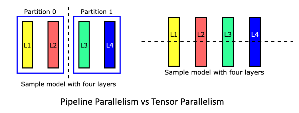
- Pipeline Parallelism (PP): Split the model by layers.
- Tensor Parallelism (TP): Split the model by individual tensors (e.g., weight matrices) within layers.
Let's dive into each of these, starting with the most common and intuitive approach: Data Parallelism.
2. Data Parallelism: More Workers, Same Blueprint
Data Parallelism is the go-to strategy when your model can fit into a single GPU's memory, but you want to speed up training by processing more data in parallel.
The Concept:
- Replicate: A complete copy of the model is placed on each GPU.
- Split: The global data batch is split into smaller micro-batches. Each GPU receives one micro-batch.
- Process: Each GPU performs a forward and backward pass on its own micro-batch, calculating gradients independently.
- Synchronize: The gradients from all GPUs are aggregated (usually averaged) across the network. This step is often called an
All-Reduceoperation. - Update: Each GPU uses the synchronized gradient to update its local copy of the model weights. This ensures all model replicas remain identical.
This is analogous to having multiple identical factories. Each factory (GPU) works on a portion of a large order (the data batch) using the same blueprint (the model). At the end of the day, they pool their findings (gradients) to improve the blueprint for the next production run.
To see this in action, the following video provides an excellent and clear animated explanation.
ChatGPT vs Thousands of GPUs! || How ML Models Train at Scale!
This video from Sourish Kundu provides an excellent overview of distributed training. We'll start with the section on Data Parallelism.
Watch the segment from 00:33 to 04:48. Focus on how the data is split, the model is replicated, and how gradients are synchronized using the 'all-reduce' operation.
Key Limitation of Data Parallelism
As the video highlights around the 4:48 mark, Data Parallelism has one major constraint: the entire model must fit into the memory of a single GPU. For models like GPT-3 or LLaMA 2 70B, this is simply not possible on most available hardware. This is the fundamental reason we need model parallelism.
3. Model Parallelism: Splitting the Model Itself
When a model is too large for one GPU, we have no choice but to split the model across multiple devices. The two main strategies for this are Pipeline Parallelism and Tensor Parallelism.
The image below provides a great high-level visual contrast between the two. Pipeline Parallelism makes "vertical" cuts between layers, while Tensor Parallelism makes "horizontal" cuts through the layers.
3.1 Pipeline Parallelism (PP): The Assembly Line
Pipeline Parallelism partitions a model "vertically" by placing contiguous blocks of layers on different GPUs.
The Concept:
- Split Layers: GPU 0 gets the first set of layers (e.g., 1-20), GPU 1 gets the next set (e.g., 21-40), and so on.
- Forward Pass: A batch of data is fed into GPU 0. After processing through its layers, the resulting activations are sent to GPU 1, which continues the forward pass. This proceeds like an assembly line down the chain of GPUs.
- The "Bubble" Problem: A naive implementation is very inefficient. While GPU 0 is working, all other GPUs are idle. When GPU 1 is working, GPU 0 and all downstream GPUs are idle. This idle time is called the "pipeline bubble."
- The Solution: Micro-batching. To reduce the bubble, the data batch is split into many smaller micro-batches. These are fed into the pipeline one after another, allowing different GPUs to be working on different micro-batches simultaneously, significantly improving utilization.
Let's watch the next segment of the video for a visual explanation.
ChatGPT vs Thousands of GPUs! || How ML Models Train at Scale!
Now, let's see how Pipeline Parallelism works and how micro-batching solves its main inefficiency.
Watch from 05:07 to 07:45. Pay close attention to the diagram showing the pipeline 'bubble' and how splitting the batch into micro-batches fills in this idle time.
Test your understanding!
Imagine you have a transformer model with 96 layers and you want to train it across 8 GPUs using Pipeline Parallelism.
- Assuming a simple, even split, how many layers would be placed on each GPU?
- In this setup, what is the key hyperparameter introduced by PP that you would need to tune to minimize the "pipeline bubble" and maximize GPU utilization?
Show answer
- Each GPU would hold
96 / 8 = 12layers. - The key hyperparameter is the number of micro-batches (sometimes called
chunksorgradient accumulation stepsin this context). A larger number of micro-batches allows for better interleaving of forward and backward passes, reducing idle time, but making the micro-batch size smaller, which can also be inefficient. Finding the sweet spot is key.
3.2 Tensor Parallelism (TP): Team-Based Computation
What if a single layer of a model is too big to fit on one GPU? This is where Tensor Parallelism comes in. Instead of splitting between layers, TP splits the computation within each layer.
The Concept:
- Split Tensors: TP splits the large weight matrices inside a model's layers (e.g., in MLP blocks or attention heads) across multiple GPUs.
- Parallel Computation: Each GPU computes a piece of the result. For a matrix multiplication
Y = XA, if the weight matrixAis split column-wise[A1, A2]across two GPUs, one GPU computesXA1and the other computesXA2. The final resultYis[Y1, Y2], which can be gathered. - Communication: This requires frequent, high-speed communication between GPUs to exchange partial results (using
All-ReduceorAll-Gathercollectives). For this reason, TP is almost exclusively used within a single machine node where GPUs are connected by a very fast interconnect like NVLink.
This approach is particularly well-suited to transformers, as the multi-head attention mechanism is inherently parallel. Each head can be computed on a different GPU.
Let's see the final conceptual piece from the video.
ChatGPT vs Thousands of GPUs! || How ML Models Train at Scale!
Tensor Parallelism is a more fine-grained approach. This last segment from the video explains how it works at the level of matrix multiplication.
Watch from 07:45 to 10:41. Focus on the distinction between column and row parallelism and how they can be chained together. Don't worry about memorizing the exact linear algebra, but grasp the core idea of splitting individual matrix operations.
4. Hybrid Strategies: Combining Paradigms for Massive Scale
In practice, training a trillion-parameter model isn't done with just one of these techniques. State-of-the-art training systems like DeepSpeed and Megatron-LM use a hybrid approach, often called 3D Parallelism, that combines all three.
A typical configuration might look like this:
- Data Parallelism (DP): Used across different machine nodes. Each node holds a slice of the overall model.
- Pipeline Parallelism (PP): Used to split the model layers across GPUs between nodes (or groups of GPUs). Communication for PP is less frequent than for TP, so it's more tolerant of slower inter-node networking.
- Tensor Parallelism (TP): Used to split layers across GPUs within a single node, taking advantage of the ultra-fast NVLink interconnect.
This combination allows for maximum flexibility in scaling both model size and training speed. The Hugging Face documentation provides an excellent guide on when to choose which strategy.
Efficient Training on Multiple GPUs
This Hugging Face guide provides a practical decision-making framework for choosing a parallelization strategy. It summarizes the concepts we've discussed and puts them into a practical context.
Please read the following sections: "Scalability strategy": This gives you a clear flowchart for deciding which paradigm to use based on your model size and hardware. "Data Parallelism + Pipeline Parallelism": Skim this to see how two paradigms are combined. "Data Parallelism + Pipeline Parallelism + Tensor Parallelism": Skim this section to understand the concept of 3D parallelism.
Summary of Paradigms
Here is a summary table to help you compare the three core paradigms:
| Paradigm | What is Split? | When to Use It? | Key Advantage | Key Disadvantage |
|---|---|---|---|---|
| Data Parallelism | The data batch | Model fits on 1 GPU, but you want to accelerate training. | Simple to implement; great for scaling training speed. | Does not solve the problem of a model being too large for a single GPU. |
| Pipeline Parallelism | The model's layers (vertically) | Model is too large for 1 GPU. | Allows training of extremely large models. | Can suffer from the "pipeline bubble" (GPU idle time); can be complex to implement. |
| Tensor Parallelism | Tensors within layers (horizontally) | A single model layer is too large for 1 GPU. | High degree of parallelism and efficient for certain architectures. | Requires very high-bandwidth interconnects between GPUs; high communication overhead. |
Conclusion
You have now surveyed the foundational strategies that make training massive language models possible. We've moved beyond single-GPU optimizations to a world of distributed computing where models and data are strategically partitioned across entire clusters of GPUs.
Key Takeaways:
- Data Parallelism (DP) is for speed: you replicate the model and split the data. It's the simplest approach but requires the model to fit on one GPU.
- Pipeline Parallelism (PP) is for size: you split the model vertically across layers, like an assembly line. It helps with memory but must be managed carefully to avoid GPU idle time.
- Tensor Parallelism (TP) is also for size, at a finer grain: you split the model horizontally, partitioning the weight matrices within layers. It's highly parallel but requires very fast communication.
- 3D Parallelism is the state of the art: it combines DP, PP, and TP to efficiently scale training to thousands of GPUs and models with trillions of parameters.
What's Next?
Over the last few modules, we have taken a deep dive into the architecture, optimization, and immense engineering effort required to train a large language model from scratch. Now, we pivot. For the rest of this course, our focus will shift from building models to using them effectively.
In our next lesson, we will begin our journey into Prompt Engineering Fundamentals. You will learn how to craft instructions that unlock the powerful capabilities of these models for a wide range of tasks, turning you from a model builder into a model commander.