Chinchilla Scaling Laws: Estimating Training Compute (FLOPs)

Introduction

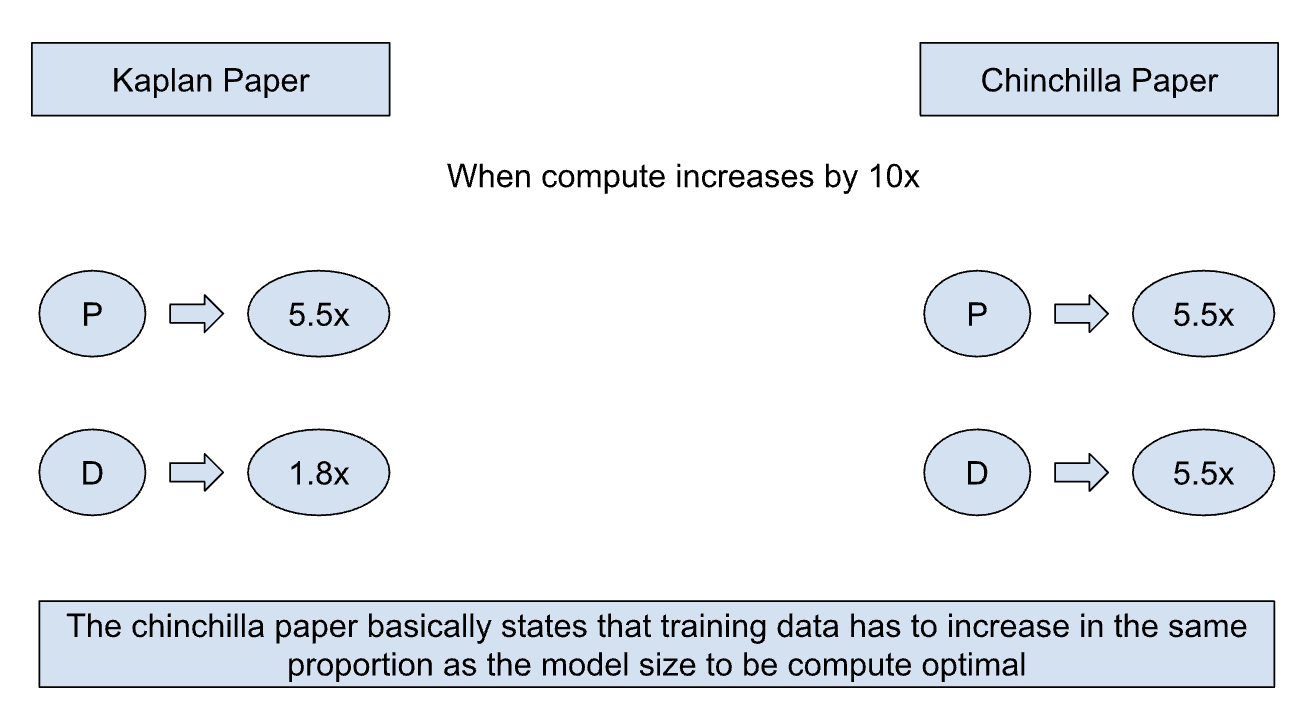
In our last lesson, we explored the paradigm shift brought about by the Chinchilla scaling laws, establishing the crucial strategic insight that for optimal training, a model's dataset size should scale proportionally with its parameter count, following the D ≈ 20N rule of thumb. We focused on the why—understanding that most large models before Chinchilla were severely undertrained.

Today, we transition from strategy to practical estimation. This lesson is designed to equip you with the tools to answer the critical questions that arise when planning a large-scale training project: "Given a specific model and dataset, how many FLOPs will it take to train?" and the reverse, "I have a compute budget of X FLOPs; what is the most efficient model and dataset size I can train?" By the end of this lesson, you will be able to estimate training compute requirements (FLOPs) for a given model and dataset size using Chinchilla scaling laws.

Part 1: The Fundamental Compute Formula

Before we can allocate a compute budget optimally, we need a way to measure it. In large-scale deep learning, the standard unit of computation is the FLOP, or Floating-Point Operation. The total compute for training a transformer model can be approximated by a surprisingly simple formula.

Chinchilla Scaling Law Overview

Let's start with the core formula that connects model size, dataset size, and compute. This brief overview defines the relationship.

Read the first paragraph of the section '1. Formulation and Interpretation'. Focus on the formula provided for the compute constraint: C ≈ 6ND.

As you just read, the total compute $C$ required to train a transformer is estimated as:

$C \approx 6 \times N \times D$

Where:

C is the total compute in FLOPs.
N is the number of parameters in the model.
D is the number of tokens in the training dataset.

The factor of 6 is a rule-of-thumb approximation. It comes from the fact that for each token processed, every parameter in the model is involved in roughly:

2 operations during the forward pass (a multiply-accumulate operation).
4 operations during the backward pass (which involves the forward pass calculations plus gradient computations, roughly doubling the work).

So, for every token, each of the $N$ parameters requires approximately $2 N + 4 N = 6 N$ FLOPs. Multiplying this by the total number of tokens $D$ gives us the total compute 6ND.

Part 2: From Compute Budget to Optimal Allocation

Now we have the two essential pieces of our puzzle:

The compute approximation: $C \approx 6 N D$
The Chinchilla-optimal ratio from our last lesson: $D \approx 20 N$

With these two equations, we can solve for the optimal model size ( $N$ ) and dataset size ( $D$ ) for any given compute budget ( $C$ ). By substituting the Chinchilla ratio into the compute formula, we get:

$C \approx 6 \times N \times (20 N)$
$C \approx 120 N^{2}$

This simple quadratic relationship is incredibly powerful. It allows us to directly calculate the optimal model size for a given compute budget.

To see this in action, let's walk through a concrete example.

Chinchilla Scaling Laws: Compute-Optimal LLM Training

This section of the 'Chinchilla Scaling Laws' article provides a clear, step-by-step worked example of calculating the optimal model and dataset size for a given compute budget. It also includes the Python code to perform this calculation, which will be very useful.

First, read the section 'Worked Example: Computing Chinchilla-Optimal Allocations'. Follow the math as it derives the optimal N and D for a budget of 10^22 FLOPs. Then, review the code in the 'Code Implementation' section. This shows how to turn the formulas into practical functions.

As the example demonstrated, by rearranging the formula to solve for $N$ , we get:

$N_{o pt} = \frac{C}{120}$

And once we have the optimal parameter count $N_{o pt}$ , finding the optimal dataset size is trivial:

$D_{o pt} = 20 \times N_{o pt}$

This calculation is the cornerstone of planning modern LLM training runs.

Test your understanding!

The original Llama 2 70B model was trained using approximately $6 \times 1 0^{23}$ FLOPs. Using the Chinchilla-optimal formulas, what would be the ideal parameter count ( $N$ ) and token count ( $D$ ) for this compute budget? How does the calculated parameter count compare to the actual 70B parameters of the Llama 2 model?

Show answer

Calculate Optimal Parameters (N):
$N_{o pt} = \frac{C}{120} = \frac{6 \times 1 0 ^{23}}{120} = 5 \times 1 0^{21} \approx 7.07 \times 1 0^{10}$
So, the optimal model size is approximately 70.7 billion parameters.
Calculate Optimal Tokens (D):
$D_{o pt} = 20 \times N_{o pt} = 20 \times (7.07 \times 1 0^{10}) \approx 1.41 \times 1 0^{12}$
So, the optimal dataset size is approximately 1.41 trillion tokens.

Comparison: The calculated optimal parameter count of ~70.7B is remarkably close to the actual Llama 2 model's 70B parameters. This is not a coincidence; the Llama family of models was designed with the Chinchilla scaling laws in mind.

Part 3: A Deeper Look at the Derivation

You now have the practical tools to perform the calculations. But to build deep mastery, it's valuable to understand how the DeepMind team arrived at the Chinchilla conclusion. They didn't just guess the D/N ≈ 20 ratio; they used three distinct and rigorous experimental methods that all pointed to the same answer.

Stanford CS336 Language Modeling from Scratch | Spring 2025 | Lecture 9: Scaling laws 1

This segment from a Stanford lecture on scaling laws provides a detailed and academically rigorous explanation of the three methods the Chinchilla paper used to find the optimal scaling relationship. This will give you the 'why' behind the formulas we're using.

Watch the segment from 53:30 to 1:00:30. The speaker walks through each of the three methods: Method 1 (Minimum Envelope): Fixing model sizes and varying data to find the optimal performance frontier. Method 2 (Isoflop Analysis): Fixing the compute budget and varying the N/D allocation to find the minimum loss. Method 3 (Parametric Fitting): Fitting a joint loss function to all the data points.

The convergence of these three different analytical approaches provides strong evidence for the validity of the Chinchilla scaling laws and is a great example of robust experimental design in large-scale ML research.

Part 4: Visualizing the LLM Landscape

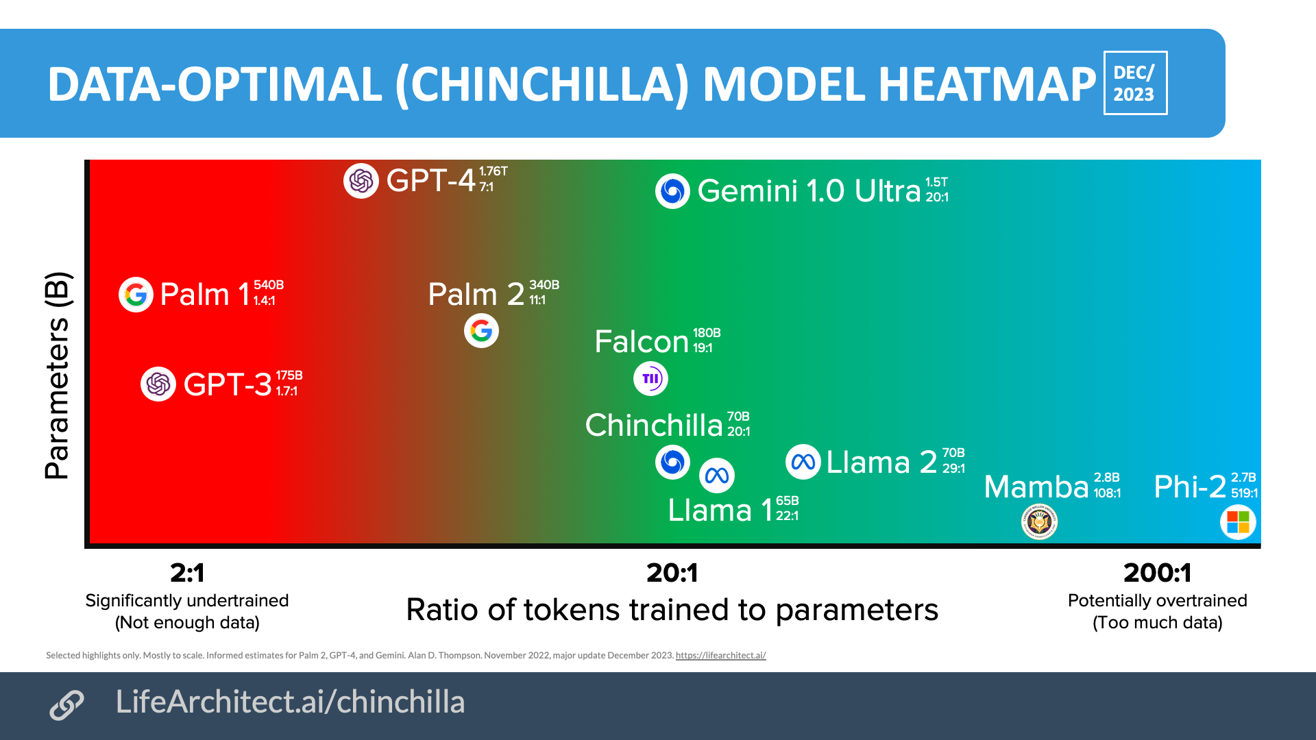
These calculations and ratios can feel abstract. A powerful way to ground them is to see where well-known models fall in relation to the Chinchilla-optimal line.

Comparison of Kaplan and Chinchilla Scaling Laws — This diagram clearly contrasts the two scaling philosophies. Kaplan's law (top) suggests that with 10x more compute, you should make the model 5.5x bigger but only use 1.8x more data. Chinchilla's law (bottom) argues for a balanced approach: with 10x more compute, you should scale both the model and the data by roughly 3.2x (since √10 ≈ 3.16, though the diagram uses 5.5x as an example from another paper, the principle of proportionality is key).

The image below plots various LLMs on a heatmap based on their parameter count and their token-to-parameter ratio. The green zone represents the Chinchilla-optimal region.

Data-Optimal (Chinchilla) Model Heatmap — This heatmap vividly illustrates the pre- and post-Chinchilla eras. Models like GPT-3 and PaLM are in the red 'undertrained' zone, with very low token/parameter ratios. In contrast, models like Chinchilla, Llama 1 & 2, and Gemini are much closer to the green 'data-optimal' band, reflecting the industry's shift in training strategy.

Test your understanding!

Looking at the heatmap, locate the GPT-3 (175B) model. It sits deep in the red "Significantly Undertrained" zone with a token/parameter ratio of less than 2:1.

Based on the Chinchilla rule of thumb, approximately how many tokens should a 175B parameter model have been trained on to be considered compute-optimal?

Show answer

Using the D ≈ 20N rule:

$D_{o pt} \approx 20 \times (175 \times 1 0^{9}) = 3500 \times 1 0^{9} = 3.5 \times 1 0^{12}$

A 175B parameter model should have been trained on approximately 3.5 trillion tokens to be Chinchilla-optimal. GPT-3 was trained on only about 300 billion tokens, which is more than 10x less than the optimal amount. This is why it's considered so undertrained.

Conclusion

Today, we've translated the strategic insights of scaling laws into concrete engineering calculations. You are no longer just aware of the Chinchilla laws; you can now apply them to estimate the resources required for LLM training and to critically evaluate the design of existing models.

Key Takeaways:

The Core Compute Formula: The training cost of a transformer can be approximated as $C \approx 6 N D$ FLOPs.
Optimal Allocation from a Budget: By combining the compute formula with the Chinchilla ratio ( $D \approx 20 N$ ), we get $C \approx 120 N^{2}$ . This allows you to determine the compute-optimal model size $N$ and dataset size $D$ for any training budget.
From Allocation to Budget: The 6ND formula allows you to calculate the total compute required if you have already decided on a model size and dataset size.
A Tool for Analysis: These calculations provide a quantitative framework for analyzing LLMs, explaining why models like Llama 2 are designed the way they are and why older models like GPT-3 were inefficient from a training compute perspective.

What's Next?

We've learned how to estimate the massive compute (FLOPs) needed for training. However, total FLOPs are just one part of the hardware challenge. The other critical bottleneck is GPU memory. How do you fit a multi-billion parameter model, its gradients, and the optimizer states into the limited VRAM of a GPU?

In our next lesson, we will tackle this question by exploring mixed-precision training (FP16 and BF16). This is a fundamental technique used in virtually all large-scale training to dramatically reduce memory usage and accelerate computations, making the enormous compute budgets we've just calculated more manageable in practice.

Recommended resources