Supervised Fine-tuning for Domain-Specific Datasets

1. The Supervised Fine-Tuning (SFT) Workflow

Supervised Fine-Tuning is the process of further training a pre-trained model on a labeled dataset to adapt its behavior for a specific task. This is distinct from pre-training (learning from vast unlabeled text) and from alignment techniques like RLHF.

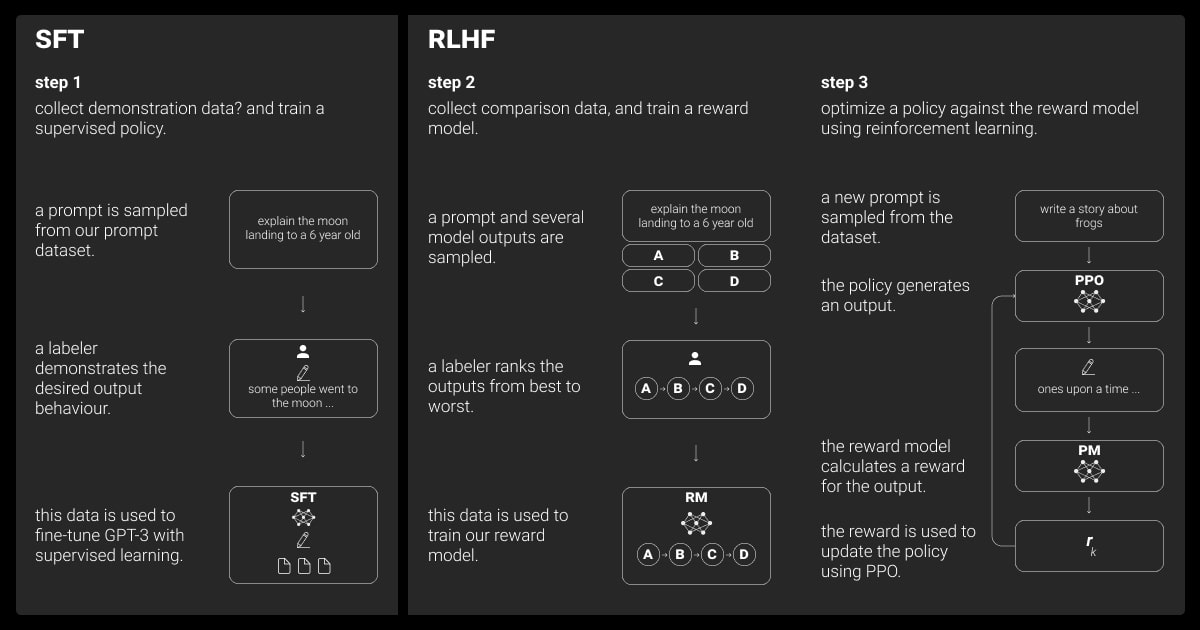
The Hugging Face trl (Transformer Reinforcement Learning) library provides a high-level API called SFTTrainer that orchestrates this entire process. To give you a roadmap for this lesson, let's look at the key steps involved in a typical SFT job.

2. Preparing the Ingredients for Training

Before we can start training, we need to prepare our data and model. While we've touched on these steps before, let's see how they fit into a practical, end-to-end script.

Dataset Preparation in Practice

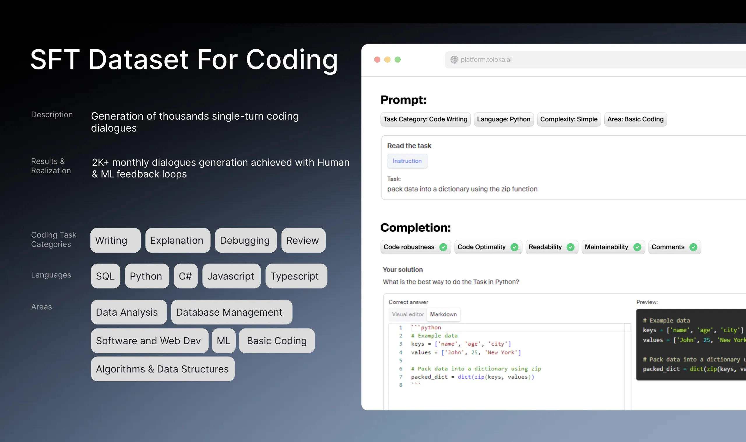
In a previous lesson, you learned how to format a dataset into prompt-completion pairs, often using the chat template format ({"messages": [...]}). A crucial part of the engineering process is transforming your raw data source (like a CSV, JSON file, or database) into this required format. This also involves practical considerations like analyzing token lengths to set an appropriate max_seq_length.

Let's see a real-world example of this process.

This data preparation phase is critical. High-quality, correctly formatted data is the single most important factor for a successful fine-tuning outcome.

Model and LoRA Configuration

Next, we set up our model. This involves loading the base model (often with quantization for memory efficiency) and defining the LoraConfig, which you mastered in the previous lesson. Let's quickly review how this looks in a complete script.

3. Configuring the Training Job with SFTTrainer

With the data and model ready, we can configure the training job itself. The SFTTrainer uses a configuration object, SFTConfig (which is an extension of TrainingArguments), to control every aspect of the training loop. Understanding these parameters is key to running stable and effective training jobs.

Let's see these parameters defined in a practical code example. The following code snippet from the Google AI Gemma fine-tuning guide shows a well-documented SFTConfig.

from trl import SFTConfig
import torch

# Assume torch_dtype is set (e.g., torch.bfloat16)
args = SFTConfig(
    # --- Job & Model Paths ---
    output_dir="gemma-text-to-sql",      # Directory to save checkpoints and repository ID
    
    # --- Dataset & Training Strategy ---
    max_seq_length=512,                 # Max sequence length (informed by your dataset analysis)
    packing=True,                       # Packs multiple short examples into one sequence for efficiency
    num_train_epochs=3,                 # Number of training epochs
    
    # --- Batching & Gradient ---
    per_device_train_batch_size=1,      # Batch size per GPU
    gradient_accumulation_steps=4,      # Accumulate gradients over 4 steps to simulate a larger batch size (1*4=4)
    gradient_checkpointing=True,        # Use gradient checkpointing to save memory
    max_grad_norm=0.3,                  # Clip gradients to prevent exploding gradients (from QLoRA paper)

    # --- Optimizer & Scheduler ---
    optim="adamw_torch_fused",          # Efficient AdamW optimizer
    learning_rate=2e-4,                 # Learning rate (a common starting point for QLoRA)
    lr_scheduler_type="constant",       # Learning rate schedule
    warmup_ratio=0.03,                  # Warmup ratio (from QLoRA paper)

    # --- Logging & Saving ---
    logging_steps=10,                   # Log metrics every 10 steps
    save_strategy="epoch",              # Save a checkpoint at the end of each epoch
    
    # --- Precision & Hardware ---
    fp16=False,                         # Set based on GPU capability
    bf16=True,                          # Set based on GPU capability

    # --- Other ---
    push_to_hub=True,                   # Push model to Hugging Face Hub
    report_to="tensorboard",            # Log to TensorBoard
)

4. Executing and Monitoring the SFT Job

Once all configurations are in place, the final steps are to instantiate the SFTTrainer and launch the training.

from trl import SFTTrainer

# Assume model, tokenizer, train_dataset, peft_config, and args are defined

# 1. Initialize the Trainer
trainer = SFTTrainer(
    model=model,
    args=args,
    train_dataset=train_dataset,
    eval_dataset=validation_dataset, # Optional: for tracking validation loss
    peft_config=peft_config,
    tokenizer=tokenizer,
)

# 2. Start the training!
trainer.train()

As the training runs, the console will output logs showing metrics like training loss, validation loss, and learning rate. Monitoring these metrics is essential for diagnosing the health of your training job.

The patterns in your loss curves can tell you a lot:

• Healthy Training: Both training and validation loss decrease and then plateau.
• Overfitting: Training loss continues to decrease, but validation loss starts to increase. The model is memorizing the training data and losing its ability to generalize.
• Underfitting: Neither training nor validation loss decreases significantly. The model doesn't have enough capacity or isn't training long enough to learn the task.

We will do a much deeper dive into interpreting these metrics in the next lesson.

5. Finalizing the Model

After the trainer.train() call completes, you have a trained adapter. You have two main options for saving and using your result.

1. Save the Adapter Only: This is the default behavior. trainer.save_model() will save the lightweight LoRA adapter weights (typically a few MB) to the specified output_dir. This is highly efficient for storage and allows you to dynamically load different adapters onto the same base model.

2. Merge and Save the Full Model: For some deployment scenarios (e.g., using inference servers like vLLM), it's easier to work with a single, merged model. You can merge the trained adapter weights back into the base model's weights and save the entire model.

This final step completes the full fine-tuning lifecycle, taking you from a raw dataset to a deployable, specialized model.

Conclusion

You have now walked through the entire workflow for configuring and executing a supervised fine-tuning job. This process is the bedrock of adapting LLMs for practical applications.

Key Takeaways:

• The SFTTrainer is your primary tool: It elegantly orchestrates the data, model, and training configurations.
• Configuration is key: The SFTConfig provides the essential knobs to control batch size, learning rate, training duration, and efficiency settings like packing and gradient_accumulation.
• The workflow is systematic: Prepare data -> configure model/LoRA -> configure training -> execute -> monitor -> save.
• Monitoring is non-negotiable: Watching the loss curves is your first line of defense against common training problems like overfitting and underfitting.
• You have deployment options: You can keep adapters separate for modularity or merge them into the base model for simplified deployment.

What's Next?

In this lesson, we saw the training logs and briefly discussed what they mean. In our next lesson, "Monitor training and validation metrics (e.g., loss, accuracy) to identify overfitting or underfitting during fine-tuning," we will perform a deep dive into this crucial diagnostic skill. You'll learn to interpret various loss patterns, understand what they imply about your model's learning process, and identify the corrective actions you can take.