Monitoring Metrics for Overfitting and Underfitting

Introduction

In our last lesson, you configured and executed a full Supervised Fine-Tuning (SFT) job. You learned how to set up the data, model, and training parameters using SFTTrainer. As the training ran, you saw logs of metrics like "training loss" and "validation loss" streaming to your console.

Today, we'll learn to become detectives. This lesson is dedicated to interpreting those metrics to diagnose the health of your fine-tuning job. You'll learn to read the "story" told by learning curves to answer the critical question: "Is my model actually learning, or is it just memorizing?" Mastering this skill is essential for an applied AI engineer. It allows you to avoid wasting expensive compute resources, debug training issues effectively, and ultimately, build models that generalize well to real-world problems. Our goal is to monitor training and validation metrics to identify overfitting or underfitting during fine-tuning.

1. The Core Metrics: Your Dashboard Instruments

Before interpreting the patterns, let's clarify what we're measuring. During fine-tuning, we evaluate the model's performance on two key data splits:

Training Set: The data the model sees during training. Performance here tells you how well the model is fitting to the data it's learning from.
Validation (or Evaluation) Set: A separate, held-out dataset the model does not train on. It's used periodically during training to check how well the model is generalizing to unseen data. This is your single most important indicator of real-world performance during the training process.

To understand these concepts and the key metrics we'll be tracking, let's watch a segment from a talk by Weights & Biases.

Training & Fine-Tuning LLMs: Evaluation

This video, 'Training & Fine-Tuning LLMs: Evaluation,' provides a clear explanation of the fundamental metrics used to monitor a language model's training progress.

Watch from 01:35 to 04:55, and then from 15:56 to 17:35. Focus on understanding: Training Loss vs. Evaluation Loss: What each represents. Cross-Entropy Loss: The intuition behind calculating loss from the model's next-token predictions. Perplexity: How it's derived from loss and what it signifies about the model's 'surprise'. The roles of the Training, Validation, and Test sets.

To summarize the key metrics:

Loss (Cross-Entropy Loss): This is the primary metric used during training. For an autoregressive model, it measures the error in its prediction of the next token. A lower loss means the model is assigning a higher probability to the correct next token. You will monitor both train_loss and eval_loss.
Accuracy: This measures the percentage of tokens the model predicted correctly. While intuitive, it can sometimes be a less sensitive measure than loss because small improvements in the model's probability distribution might not be enough to change the final predicted token, leaving accuracy unchanged.
Perplexity (PPL): Often reported in academic papers, perplexity is the exponentiation of the cross-entropy loss ( $PPL = e^{loss}$ ). Intuitively, it measures how "confused" or "perplexed" the model is by the data. A perplexity of 20, for example, means that at each token, the model is as uncertain as if it had to choose uniformly among 20 possibilities. Lower is better.

2. Interpreting Learning Curves: Diagnosing Training Health

These metrics are typically plotted over training steps or epochs to create learning curves. Your ability to interpret the shape of these curves is what transforms you from someone who simply runs training scripts to an engineer who can debug and improve them.

Let's dive into the most common patterns you'll encounter. The following article from the Hugging Face LLM Course is an excellent reference for this section.

Understanding Learning Curves - Hugging Face LLM Course

The article 'Understanding Learning Curves' from the Hugging Face LLM Course provides a fantastic visual guide to interpreting these plots. We will use it to understand the different training scenarios.

Read the introduction ('What are Learning Curves?'), and then focus on the sections 'Healthy Learning Curves,' 'Overfitting,' and 'Underfitting.' Pay close attention to the visual examples of the loss curves for each case and the proposed solutions.

Let's break down the key scenarios.

Scenario 1: The "Healthy" Fit

This is the ideal outcome. The model learns the general patterns in the data without memorizing the noise.

Training and Validation Loss over Epochs: Underfitting, Right Fit, and Overfitting — This image compares three training scenarios. The middle plot, 'Right Fit,' illustrates a healthy training run where both training and validation loss decrease and converge to a low value with a minimal gap between them.

Symptoms:

Both train_loss and eval_loss decrease steadily.
The curves converge, or "flatten out," at a low value.
The gap between the train_loss and eval_loss is small and stable.

This indicates your model has successfully generalized from the training data.

Scenario 2: Overfitting

This is the most common problem you'll face. The model learns the training data too well, including its noise and specific quirks, and loses its ability to generalize to new, unseen examples.

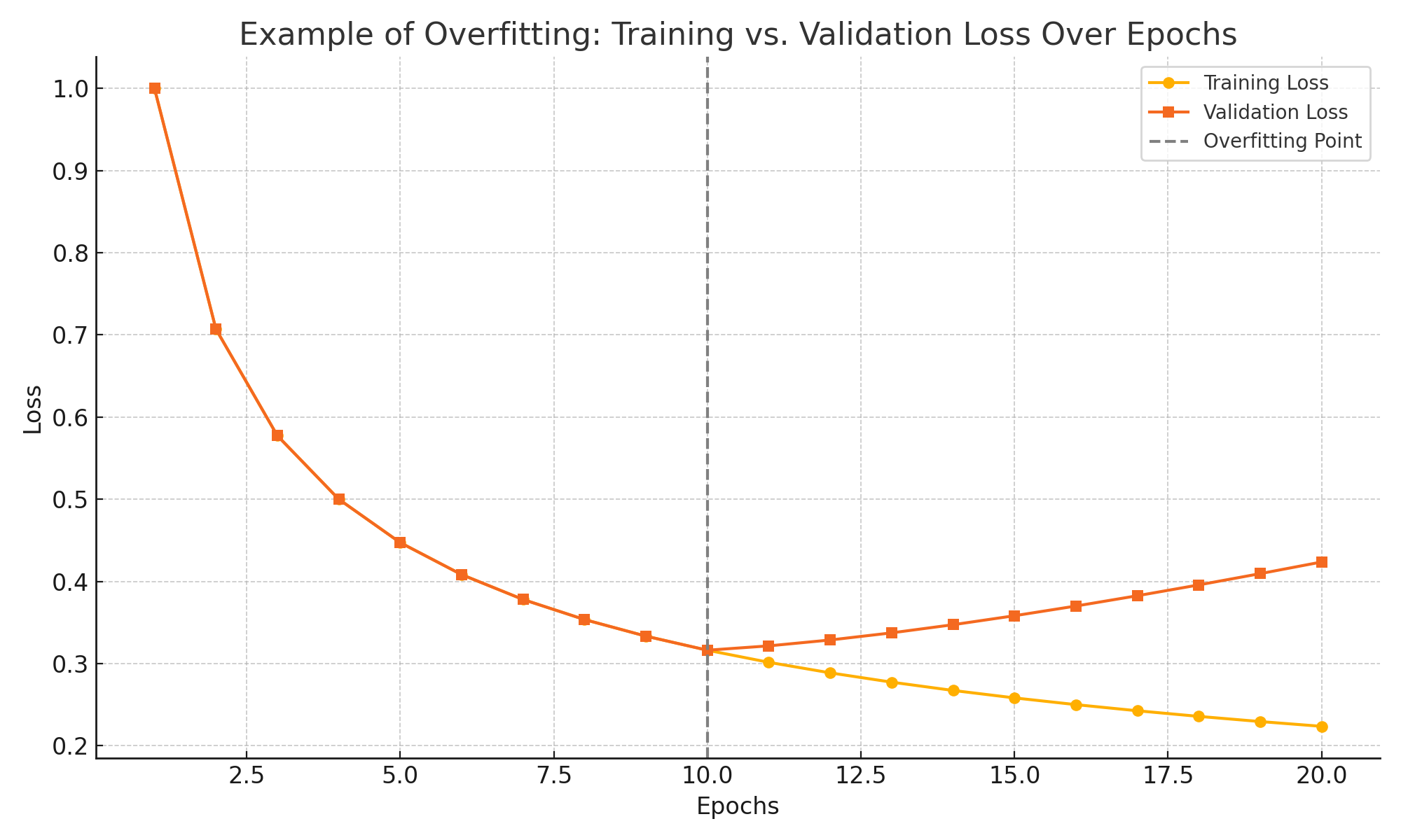
Example of Overfitting: Training vs. Validation Loss Over Epochs — This plot shows a classic case of overfitting. The training loss (yellow) continues to decrease, while the validation loss (orange) begins to rise. The point where the validation loss is at its minimum is the optimal stopping point.

Symptoms:

train_loss continues to decrease.
eval_loss initially decreases but then stagnates or, worse, starts to increase.
A significant and growing gap appears between your training and validation metrics.

Solutions:

Early Stopping: This is your first line of defense. Stop the training process at the point where the eval_loss is at its minimum, before it starts to rise. Most training frameworks, including Hugging Face's Trainer, have built-in support for this.
Reduce Training Time: Train for fewer epochs.
Add More/Better Data: A larger, more diverse training set makes it harder for the model to simply memorize everything.
Use Regularization: Techniques like dropout or weight decay discourage the model from relying too heavily on any single feature. In PEFT, you can also try reducing the LoRA rank (r), which reduces the number of trainable parameters.

Scenario 3: Underfitting

This occurs when the model is not complex enough or hasn't trained long enough to capture the underlying patterns in the data.

Symptoms (from the 'Underfitting' plot in the first image):

Both train_loss and eval_loss remain high and fail to decrease significantly.
The curves plateau at a high loss value early in training.
The model performs poorly on both the training and validation sets.

Solutions:

Train Longer: Increase the number of num_train_epochs.
Increase Model Capacity: If using PEFT, you could increase the LoRA rank (r) to give the model more parameters to work with. In more extreme cases, you might need to use a larger base model.
Adjust Learning Rate: Your learning rate might be too low, causing training to proceed too slowly.
Check Data Quality: Ensure your data is clean and relevant to the task. If the data is too noisy, the model may struggle to find a meaningful signal.

Test your understanding!

You are fine-tuning a Llama 3 model. After 3 epochs, you observe the following metrics:

train_loss: 0.25
eval_loss: 0.85
train_accuracy: 0.95
eval_accuracy: 0.70

In the first epoch, the eval_loss was 0.75. What is the most likely problem, and what is your immediate first action?

Show answer

The most likely problem is overfitting. The large gap between training metrics (loss 0.25, accuracy 95%) and evaluation metrics (loss 0.85, accuracy 70%) is a classic symptom. Furthermore, the eval_loss has increased from 0.75 in the first epoch to 0.85 in the third, which is a definitive sign.

Your immediate first action should be to implement early stopping based on eval_loss. You would re-run the training and configure it to save the model checkpoint from the epoch with the lowest eval_loss (in this case, likely epoch 1 or 2) and stop training once the eval_loss stops improving for a certain number of evaluation steps.

3. Monitoring in Practice with Tooling

Theory is great, but as an engineer, you'll be working with tools that make this process tangible. Experiment tracking platforms like Weights & Biases (W&B) are industry standard for visualizing these curves and other system metrics in real-time.

Let's see what this looks like in a real fine-tuning project.

Training & Fine-Tuning LLMs: Introduction

The following demo from the Weights & Biases 'Training & Fine-Tuning LLMs' course shows a hands-on example of monitoring a fine-tuning job comparing Falcon-7B and Llama2-7B. This is exactly what you would do in a real-world project.

Watch from 45:22 to 59:00, and then briefly from 01:03:00 to 01:05:00. This is a longer segment, but it's packed with practical insights. Focus on: The W&B Dashboard: How loss curves for different models (Llama2 vs Falcon) are plotted and compared. Diagnosing Training: The speaker observes that Llama 2 has a better (lower) loss curve, indicating it's learning more effectively on the same data. System Metrics: Notice how he inspects GPU utilization and memory. He points out that utilization isn't 100%, suggesting a potential data loading bottleneck. This is a top-tier engineering insight—diagnosing not just the model, but the entire pipeline. Evaluation Results: The speaker evaluates the base and fine-tuned models on benchmarks, showing how fine-tuning doesn't always improve every metric (e.g., arithmetic performance dropped), which highlights the importance of data quality and targeted evaluation.

This practical demonstration reinforces that monitoring is an active, diagnostic process. You're not just watching a line go down; you're correlating model performance with system performance to build a holistic understanding of your training job.

Conclusion

In this lesson, you've moved from simply running a training script to actively diagnosing its performance. You are now equipped to identify the critical signs of a healthy training run, as well as the tell-tale symptoms of overfitting and underfitting.

Key Takeaways:

Learning curves tell a story: The relationship between training loss and validation loss is your guide to a model's generalization ability.
Overfitting is your primary adversary: A decreasing train_loss with a rising eval_loss means your model is memorizing, not learning. Early stopping is your best friend.
Underfitting means more work is needed: High loss on both train and validation sets indicates your model needs more capacity, more training time, or better data.
Monitoring is a holistic process: Beyond loss curves, monitoring system metrics like GPU utilization can help you identify and fix bottlenecks in your training pipeline, leading to more efficient fine-tuning.

What's Next?

You now know how to diagnose common training problems by looking at the metrics. But how do you systematically fix them? Many of the solutions involve changing hyperparameters related to the fine-tuning method itself. In our next lesson, we will dive into "key hyperparameters for PEFT (e.g., rank, alpha) and strategies for their optimization." You will learn how to tune these specific knobs to control model capacity and prevent the very issues you've learned to identify today.

Recommended resources