Welcome to your second lesson! We're building directly on what we established last time about the shift from statistical to neural language models.
In our previous lesson, we saw how even a simple neural network could replicate the function of a statistical bigram model. However, we used a crude method called one-hot encoding to represent characters. This method is inefficient and, more importantly, treats every word (or character) as a completely isolated entity, failing to capture any notion of similarity. Today, we solve that problem by introducing word embeddings, the first major step towards giving our models a true sense of language semantics.
Our goal is to implement a simple word embedding layer and explain its role in capturing meaning. By the end of this lesson, you'll understand how words are transformed into rich numerical representations and how these representations form the foundation of all modern NLP models.
From Isolated Points to a Semantic Space
One-hot vectors, which we used previously, are sparse, high-dimensional, and orthogonal. The orthogonality means the dot product between any two distinct word vectors is zero, mathematically enforcing the idea that they have no relationship. "King" is no more related to "Queen" than it is to "Tractor". This is a major limitation.
The solution is to represent words not as isolated points in a sparse space, but as dense vectors in a lower-dimensional semantic space. In this space, the position of a vector encodes the word's meaning.
To build intuition, let's start with a thought experiment.
This tutorial, 'Word Embedding Demo', provides a fantastic non-technical introduction to the idea of a semantic feature space. It starts by manually defining features before showing why we need to learn them.
Read the sections 'Semantic Feature Space', 'Uses of Semantic Feature Vectors', and 'Word Embeddings'. Focus on how words can be plotted as coordinates and how vector arithmetic can be used to solve analogies. Pay attention to the transition from hand-crafted features to machine-learned embeddings.
As you just read, we can imagine a space where dimensions correspond to semantic attributes like gender, age, or royalty.
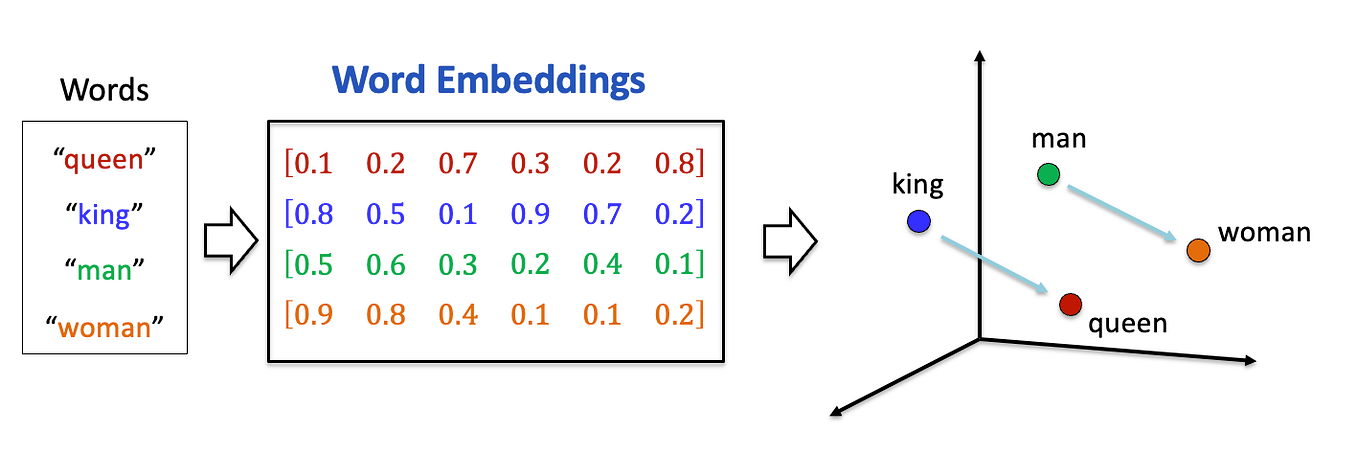
The crucial leap for modern NLP was realizing that we don't have to manually define these semantic dimensions. Instead, we can let a neural network learn them automatically. This is possible due to a key linguistic principle.
The Distributional Hypothesis: The "Why" Behind Embeddings
The idea that a neural network can learn meaningful word vectors is grounded in the distributional hypothesis, which states:
Words that appear in similar contexts tend to have similar meanings.
For example, the words "cat" and "dog" frequently appear in contexts like "the ___ is playing," "I pet the ___," or "a bowl of ___ food." By analyzing a massive amount of text, a model learns that "cat" and "dog" are interchangeable in many contexts. Therefore, it will push their vector representations close together in the semantic space it is building.
This is the core principle that allows embeddings to be learned, rather than hand-engineered.
To delve deeper into this concept and see how it's framed in the context of PyTorch, let's turn to the official documentation.
Word Embeddings: Encoding Lexical Semantics
This official PyTorch tutorial, 'Word Embeddings: Encoding Lexical Semantics', provides the theoretical motivation for word embeddings and then shows how to implement them.
Read the introductory section up to (but not including) 'Word Embeddings in Pytorch'. This reinforces the limitations of one-hot encoding and explains how dense, learnable embeddings solve the problem.
Implementing Word Embeddings in PyTorch
Now that we understand the "what" and "why," let's focus on the "how." In PyTorch, word embeddings are handled by the torch.nn.Embedding layer.
Conceptually, you can think of this layer as a simple lookup table. It's a matrix where each row is the vector representation for a single word in our vocabulary.

The nn.Embedding layer is initialized with two main arguments:
num_embeddings: The size of your vocabulary (i.e., the number of unique words).embedding_dim: The size of the dense vector you want to use for each word (e.g., 50, 100, 300).
The weights of this lookup table are initialized randomly but are then treated as trainable parameters. During training, the model receives gradients for the embedding vectors and updates them via backpropagation, just like any other parameter in the network. This is how the embeddings are learned.
Let's look at the basic usage.
Word Embeddings: Encoding Lexical Semantics
We'll now continue with the same PyTorch tutorial to see how the nn.Embedding layer is used in code.
Read the short section 'Word Embeddings in Pytorch'. Pay close attention to how you create the layer and how you use a LongTensor of indices to retrieve the embeddings.
Application: A Neural N-Gram Model with Embeddings
Let's put this all together. We will now build a neural N-Gram language model, which directly improves upon the models from our last lesson. Instead of using one-hot vectors, we'll use an nn.Embedding layer.
The task remains the same: predict the next word given the previous N words. Here's how the model will work:
- Take the integer indices of the
Ncontext words. - Look up their corresponding embedding vectors using the
nn.Embeddinglayer. - Concatenate these vectors into a single, larger vector.
- Pass this concatenated vector through one or more linear layers.
- The final output will be a vector of logits, which is passed through a
log_softmaxfunction to get the log probabilities for every word in the vocabulary.
The following resource provides the complete, runnable code for this model. Since you're already comfortable with PyTorch, focus on the NGramLanguageModeler class definition and the training loop logic.
Word Embeddings: Encoding Lexical Semantics
This final section of the PyTorch tutorial provides a complete example of using embeddings in a neural language model. It's the perfect bridge from our last lesson to this one.
Read and analyze the code in the section 'An Example: N-Gram Language Modeling'. Trace the data flow inside the forward method: from input indices, to embeddings, to concatenated vectors, and finally to output log probabilities. Notice how the embedding matrix is part of the model and thus its weights are learned during training.
By using embeddings, this model can now generalize. If it learns "the cat sat on the mat," it can infer that "the dog sat on the mat" is also a plausible sentence, because the vectors for "cat" and "dog" will be similar. This overcomes a key failure of both statistical n-grams and our one-hot-based neural model from the last lesson.
Test your understanding!
In the NGramLanguageModeler example, the model has an embedding layer defined as self.embeddings = nn.Embedding(vocab_size, embedding_dim).
If your vocabulary has 10,000 words and you choose an embedding_dim of 300, how many trainable parameters does this single embedding layer contribute to the model?
Show answer
The nn.Embedding layer is a lookup table of size vocab_size x embedding_dim. Each value in this table is a trainable parameter.
Therefore, the total number of parameters is 10,000 * 300 = 3,000,000. This highlights that the embedding layer often contains the vast majority of parameters in simpler NLP models.
Conclusion
In this lesson, we made a significant leap from representing words as isolated symbols to representing them as rich, learned vectors.
Key Takeaways:
- Word embeddings are dense, low-dimensional vectors that capture the semantic meaning of words.
- They solve the major shortcomings of one-hot encoding (high dimensionality, sparsity, and lack of similarity).
- The learning process is guided by the distributional hypothesis: words in similar contexts get similar vector representations.
- In PyTorch, the
nn.Embeddinglayer acts as a learnable lookup table, mapping word indices to their corresponding vectors. - These learned embeddings allow models to generalize based on semantic similarity, a critical capability for understanding language.
You have now grasped a fundamental building block of all modern LLMs. Every complex architecture we will study, from RNNs to Transformers, begins with an embedding layer to convert input text into a meaningful numerical format.
What's Next?
Our neural n-gram model, while an improvement, still has a rigid, fixed-size context window (e.g., it only looks at the last 2 words). To handle sequences of arbitrary length and capture longer-range dependencies, we need a more dynamic architecture.
In the next lesson, we will introduce the Recurrent Neural Network (RNN). You will learn about the sequence-to-sequence architecture and its encoder-decoder paradigm, which was the dominant approach for tasks like machine translation before the arrival of the Transformer.