From N-grams to Neural Language Models

What is a Language Model?

At its core, a language model (LM) is a system that calculates the probability of a sequence of words. A primary task for an LM is to predict the next word (or, more technically, token) in a sequence, given the words that came before it. You see a simple version of this every day with your phone's autocomplete feature.

Formally, given a sequence of words $w_1,w_2,...,w_{t-1}$, the model aims to compute the probability distribution over the entire vocabulary for the next word, $w_t$:

This seemingly simple prediction task is the foundation upon which almost all modern Natural Language Processing (NLP) is built. A model that can do this well has implicitly learned the grammar, semantics, and common sense of a language.

The Statistical Era: N-Gram Models

The earliest successful language models were statistical. They didn't "understand" language in a human sense; instead, they relied on counting word frequencies in massive text corpora. The most common approach was the n-gram model.

To get a quick and clear overview of n-grams, from unigrams to bigrams, please watch the first few minutes of the following video.

As the video explained, an n-gram model makes a simplifying assumption known as the Markov assumption: the probability of the next word depends only on the previous n-1 words.

• A bigram model (n=2) assumes the probability of a word depends only on the single word that precedes it: $P(w_t|w_1,...,w_{t-1})\approx P(w_t|w_{t-1})$.
• A trigram model (n=3) uses the two preceding words: $P(w_t|w_1,...,w_{t-1})\approx P(w_t|w_{t-2},w_{t-1})$.

These probabilities are calculated using Maximum Likelihood Estimation (MLE), which is just a formal way of saying "count and divide":

For a more detailed summary of n-grams and their critical limitations, please read the first part of the following article.

The Downfall of N-grams

As you just read, while n-gram models were simple and effective for certain tasks, they had fundamental flaws that prevented further progress:

1. Data Sparsity: If a valid bigram (e.g., "machine learning") never appeared in your training text, the model would assign it a probability of zero. This means the model is incapable of generating novel yet plausible phrases. Techniques like smoothing were developed to mitigate this, but they are essentially patches on a flawed foundation.
2. Limited Context: An n-gram model has a fixed and very small context window (typically n=2 or 3). It cannot capture long-range dependencies. Consider the sentence: "The man who grew up in France and lived there for 20 years speaks fluent ___." A bigram model only sees "fluent" and has no idea that "France" appeared much earlier.
3. No Semantic Understanding: The model treats words as discrete, isolated symbols. It has no concept that "dog" and "puppy" are semantically similar. If it learned "the cute dog," it has no way to generalize that knowledge to "the cute puppy."

These limitations created a ceiling for what was possible with statistical methods, paving the way for a new paradigm: neural language models.

The Shift to Neural Language Models

Instead of just counting co-occurrences, neural networks approach language modeling as a learning problem. The goal is still to predict the next word, but the method is fundamentally different. This new approach directly addresses the shortcomings of n-grams by learning continuous representations of words (known as word embeddings) that capture semantic meaning.

To see this evolution in action, we will now dive into a hands-on example from Andrej Karpathy's "makemore" series. This video is exceptional because it builds a simple character-level bigram model in two ways:

1. The "classic" statistical way (counting and normalizing).
2. The modern neural network way (gradient-based optimization).

By the end, you will see that both approaches can solve the same simple problem, but the neural approach is infinitely more flexible and scalable, which is why it has taken over the field. Given your experience with PyTorch, you will be able to follow the implementation details closely.

Deep Dive: From Counting to Learning

We will walk through the video in stages. The core idea is to build a character-level model to generate name-like words.

Part 1: The Statistical Bigram Model

First, let's see how to build a bigram model by counting. In this section, Karpathy loads the data, counts character pairs, stores them in a PyTorch tensor, and normalizes the counts to get probability distributions. He then samples from these distributions to generate new names.

Part 2: The Neural Network Reframing

Now for the crucial shift. Karpathy reframes the exact same problem in a neural network framework. Instead of explicitly counting, we will define a model whose parameters (weights) we can optimize to learn the probabilities.

This section covers:

• Creating a training set of input-output pairs ((character_1, character_2)).
• One-hot encoding the input character to feed it into a network.
• Defining the simplest possible neural network: a single linear layer, which is just a weight matrix W.
• Applying the softmax function to the output of the linear layer (the "logits") to produce a valid probability distribution.

Notice the key insight here: when you multiply a one-hot encoded vector by a weight matrix W, you are effectively just selecting a specific row from W. This means the weight matrix W is serving a similar role to the count-based table we built earlier, where each row corresponds to a starting character.

Part 3: Optimization and The Big Connection

We now have a model and a way to get probabilities from it. But how do we find the right values for our weight matrix W? We use gradient descent.

This final section shows how to:

• Calculate the negative log-likelihood of the correct next characters. This is our loss function.
• Perform the backward pass to get the gradients of the loss with respect to W.
• Update W to minimize the loss.
• Finally, Karpathy reveals the beautiful connection: the optimized W from the neural network is mathematically equivalent to the log-counts from the statistical model. The neural network learned the statistical properties of the data.

The key takeaway is that while the statistical approach is simple and direct for this bigram case, it's a dead end. We cannot feasibly create a "count table" for a 10-gram model because the number of possible 9-word prefixes is astronomical. The neural network framework, however, is incredibly flexible. We can make the network more complex to handle more context without changing the fundamental process of optimization via gradient descent. This scalability is what enabled the transition to more powerful models.

Conclusion

In this lesson, we traced the critical first step in the evolution of language models.

• We started with statistical n-gram models, which predict the next word by counting occurrences in a text corpus.
• We identified their fundamental limitations: data sparsity, a rigid and short context window, and an inability to understand semantic similarity.
• We then saw how the problem could be reframed in a neural network framework. By representing inputs and learning weights through gradient descent, a neural model can learn the same statistical patterns.
• Most importantly, we established that this neural framework, while equivalent in the simplest case, is far more scalable and flexible, opening the door to the complex architectures that power modern LLMs.

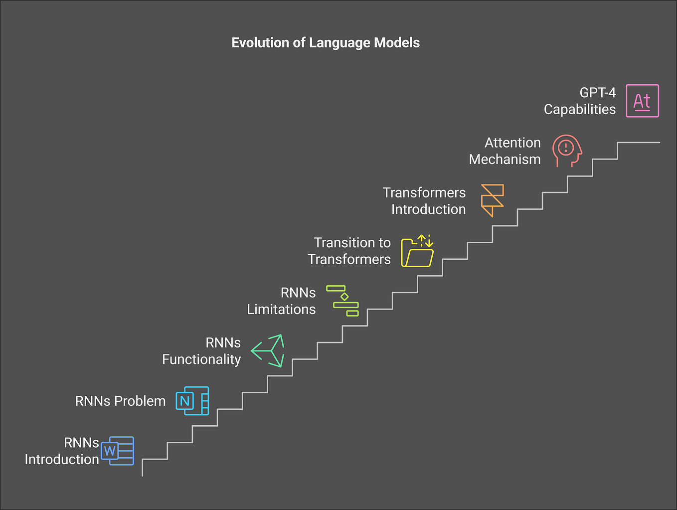
This first step on the staircase of language models is complete.

What's Next?

In the neural network we just explored, we used a simple one-hot vector -> weight matrix lookup. This is a crude way of representing words. The next major breakthrough was the development of word embeddings, which are dense vector representations that capture the rich semantic relationships between words.

In our next lesson, you will implement a simple word embedding layer and explain its role in capturing semantics. This is the next logical step from what we learned today and a core building block for all subsequent models.