Hello! Welcome to your third lesson.
In our last session, we upgraded our language models by replacing inefficient one-hot vectors with word embeddings. This allowed our model to understand semantic relationships between words, but it still suffered from a major constraint: a fixed-size context window. It could only look at a predefined number of previous words, which is a significant limitation for understanding the full context of a sentence.
Today, we'll break free from that constraint. We will explore the sequence-to-sequence (seq2seq) architecture, a powerful framework that uses Recurrent Neural Networks (RNNs) to handle inputs and outputs of variable lengths. This architecture was a cornerstone of modern NLP, particularly for machine translation, and understanding it is essential before we move on to the Transformer.
Our learning outcome is to describe the sequence-to-sequence architecture and its encoder-decoder paradigm using RNNs. By the end of this lesson, you'll understand how to process an entire input sequence into a single "thought" and then generate a new sequence from it.
The Challenge of Variable-Length Sequences
Many real-world NLP problems don't have a fixed input-to-output mapping. Consider machine translation:
- "How are you?" (3 words) -> "¿Cómo estás?" (2 words)
- "Let's go." (2 words) -> "Vamos." (1 word)
The input and output sequences have different lengths, and there isn't a simple one-to-one alignment between them. The N-gram model we built is fundamentally incapable of handling this. We need an architecture that can consume a sequence of any length and generate another sequence of any length.
The Encoder-Decoder Paradigm
The solution is the encoder-decoder architecture, the core of seq2seq models. It consists of two main components:
-
The Encoder: This is an RNN that reads the input sequence one token at a time. Its job is to process the entire sequence and compress its meaning into a fixed-size numerical representation called the context vector (sometimes called a "thought vector"). This vector is the final hidden state of the encoder RNN.
-
The Decoder: This is another RNN that takes the context vector from the encoder and generates the output sequence one token at a time. It uses the context vector to "prime" its initial state, giving it the full context of the input sequence.
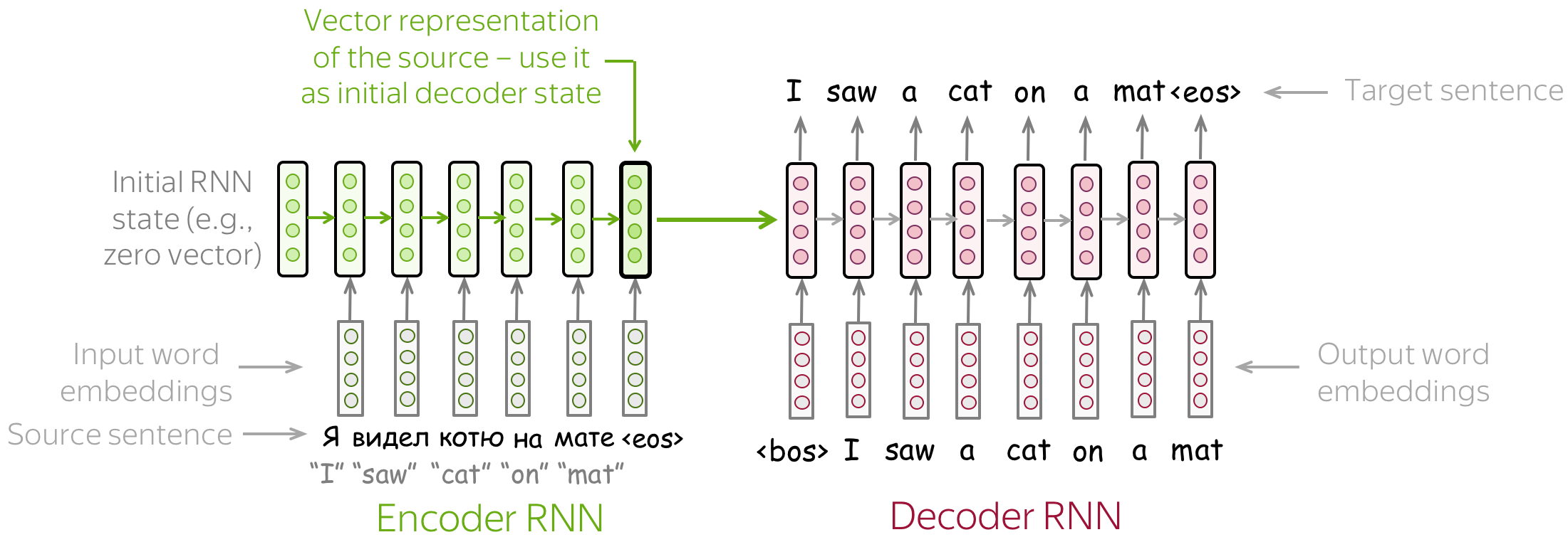
To get a dynamic feel for this process, the illustrations in the following blog post are excellent.
Visualizing A Neural Machine Translation Model
The post 'Visualizing A Neural Machine Translation Model' by Jay Alammar provides some of the clearest visual explanations of the seq2seq architecture. The animated diagrams really help build intuition.
Read the sections 'Looking under the hood' and the unlabelled section that follows, ending just before 'Let's Pay Attention Now'. Focus on the animated diagrams showing the encoder processing the input and passing the final context vector to the decoder.
A Deeper Look at the Architecture
Now that we have the high-level picture, let's zoom in on how the encoder and decoder work internally using RNNs (specifically, LSTMs or GRUs, which are advanced RNN variants we'll discuss soon).
The following video provides a clear, step-by-step walkthrough of the entire process, from embedding the input tokens to generating the final output sequence.
Sequence-to-Sequence (seq2seq) Encoder-Decoder Neural Networks, Clearly Explained!!!
The StatQuest video, 'Sequence-to-Sequence (seq2seq) Encoder-Decoder Neural Networks, Clearly Explained!!!', does a fantastic job of breaking down the architecture. It covers the roles of the embedding layers, the multi-layer RNNs, the context vector, and the final output layer.
Watch the sections that detail the construction of the encoder (3:53-8:17) and the decoder (8:17-12:03). Pay close attention to: How the final hidden states of all encoder layers form the context vector. How this context vector is used to initialize the decoder's hidden states. The autoregressive nature of the decoder: how the output of one step becomes the input for the next.
As you saw in the video, the key steps are:
- Encoder: The input sequence is embedded and fed into the encoder RNN. The final hidden state(s) become the context vector.
- Context Transfer: The context vector is used as the initial hidden state for the decoder RNN.
- Decoder:
- Starts with a special beginning-of-sequence (
<BOS>or<start>) token. - At each step, the decoder RNN outputs a hidden state. This is passed through a final linear layer and a softmax function to predict the next token in the output sequence.
- The predicted token is then fed as the input to the next time step.
- This process repeats until an end-of-sequence (
<EOS>) token is generated.
- Starts with a special beginning-of-sequence (
Training vs. Inference: The Role of Teacher Forcing
There is a crucial difference between how a seq2seq model is trained and how it's used for inference (prediction).
During inference, the model behaves exactly as described above, feeding its own predictions back into the next step.
However, during training, relying on the model's own (initially random) predictions can make training slow and unstable. A small error at the beginning can cascade and throw off the entire rest of the sequence. To solve this, we use a technique called teacher forcing.
With teacher forcing, during training, we always feed the correct ground-truth token from the target sequence as input to the next decoder step, regardless of what the model predicted. This provides a stable signal and helps the model learn to generate the correct sequence much more effectively.
Test your understanding!
Imagine you are training a seq2seq model to translate "I am fine" to "je vais bien". At the first decoding step, the model should predict "je", but it incorrectly predicts "suis".
Without teacher forcing, what token would be fed into the second decoding step? With teacher forcing, what token would be fed? What is the primary benefit of the latter approach?
Show answer
- Without teacher forcing: The model's incorrect prediction, "suis", would be fed as input to the second decoding step.
- With teacher forcing: The correct ground-truth token, "vais", would be fed as input to the second step, ignoring the model's mistake.
The primary benefit of teacher forcing is training stability and efficiency. It prevents errors from compounding and ensures that the model is always learning from a correct context at each step, leading to faster convergence.
The next video provides a very thorough walkthrough of the entire training process, including data preparation, the forward pass, loss calculation, and a great explanation of teacher forcing.
Encoder Decoder | Sequence-to-Sequence Architecture | Deep Learning | CampusX
The video 'Encoder Decoder | Sequence-to-Sequence Architecture' from CampusX gives a detailed perspective on training and inference.
Watch the following three segments: Architecture Details (13:52 - 19:08): This reinforces how LSTMs are used in the encoder and decoder. Training Process & Teacher Forcing (19:21 - 40:10): Focus on the segment from 31:40 to 35:00, which specifically explains and visualizes teacher forcing. The rest of this long section details the full forward pass with loss calculation, which is also valuable context. Prediction/Inference (48:43 - 55:25): This shows how the trained model generates output without teacher forcing.
From Concepts to Code
Given your background in PyTorch, it's useful to see how this architecture is implemented. The resource below provides a complete implementation using GRUs (a type of RNN similar to LSTMs). Don't worry about understanding every line of code, but focus on the structure.
Sequence-to-Sequence Learning for Machine...
The 'Dive into Deep Learning' chapter on seq2seq provides a comprehensive look at the architecture, complete with code. This will help connect the diagrams and videos to a concrete implementation.
Skim through the sections 'Encoder', 'Decoder', and 'Encoder–Decoder for Sequence-to-Sequence Learning'. In the PyTorch code blocks, notice: The Seq2SeqEncoder class takes a sequence and returns a final state (enc_state). The Seq2SeqDecoder class is initialized with the encoder's state. Inside the decoder's forward method, the context is concatenated with the input embeddings at each step, providing a constant reminder of the source sentence.
Conclusion
Today you've learned about the powerful sequence-to-sequence architecture, which was a revolutionary step in NLP.
Key Takeaways:
- Seq2seq models solve the problem of mapping variable-length input sequences to variable-length output sequences.
- The encoder, an RNN, processes the input and compresses its meaning into a fixed-size context vector.
- The decoder, another RNN, uses this context vector to generate the output sequence one token at a time in an autoregressive fashion.
- Teacher forcing is a crucial training technique that stabilizes learning by feeding the correct target tokens to the decoder, rather than its own, possibly flawed, predictions.
- The primary weakness of this architecture is the context vector bottleneck—the entire meaning of the input must be squeezed into one fixed-size vector.
This bottleneck is a major limitation, especially for long sequences. If the input sentence is 100 words long, the model has to cram all of that information into the same size vector as if the sentence were 10 words long. This leads to information loss and is a key motivation for the developments we will explore next.
What's Next?
The simple RNNs we've alluded to suffer from a critical flaw known as the vanishing and exploding gradient problems. This makes it very difficult for them to learn long-range dependencies, compounding the context vector bottleneck issue.
In our next lesson, we will dive into these gradient problems to understand exactly why they occur in RNNs. This will set the stage for understanding the architectural innovations—LSTMs and GRUs—that were created specifically to solve them.