Welcome back. In our last lesson, we customized the calculations in our PivotTables, learning to switch between Sum, Count, and Average to answer more nuanced analytical questions. Now that you can control what is being calculated, we'll focus on how the data is organized over time.
This lesson addresses a cornerstone of financial analysis: trend reporting. We will explore how to group your PivotTable data by different date periods like months, quarters, and years. Mastering this skill will enable you to transform a long list of transactions into a clear, high-level summary of performance over time—a fundamental task for any accounting professional preparing monthly or quarterly reports.
Automatic Date Grouping: Excel's Intelligent Assistant
One of the most powerful features of modern Excel is its ability to automatically understand and group dates. When you have a column of dates in your source data and you drag that date field into the Rows or Columns area of your PivotTable, Excel doesn't just list every single day. Instead, it intelligently groups them.
In Excel 2016 and newer versions, dragging a date field typically creates a hierarchy, automatically adding fields for Years, Quarters, and Months.
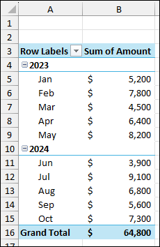
This automatic grouping is incredibly useful for getting a quick overview of your data across different time frames. You can click the + or - icons next to the year to expand or collapse the view, allowing you to drill down from an annual total to see the monthly details.
The following short video clip demonstrates this automatic grouping in action.
Excel Year-Over-Year and Period-Over-Period Analysis with PivotTables
This video from Chris Menard's YouTube channel provides a very clear demonstration of how Excel automatically groups dates when they are added to a PivotTable.
Watch the segment from the initial grouping. Notice how dragging the 'Date' field into the Rows area instantly creates a hierarchy of Years, Quarters, and Months.
Taking Control: Manual and Custom Date Grouping
While automatic grouping is a great start, you will often need to customize the report to fit specific analytical needs. For instance, you might want to compare performance by month and year but exclude quarters, or you might want to see data aggregated only by quarter to analyze seasonality.
To do this, you first need to know how to remove Excel's default grouping. You can do this in two ways:
- Immediately after dragging the date field, press
Ctrl + Z. - Right-click on any of the date labels (e.g., a year or month) in the PivotTable and select Ungroup.
Once ungrouped (or if you want to change the existing grouping), you can apply your own. Right-click on any date and select Group. This opens the Grouping dialog box, where you have full control.
The Grouping dialog box allows you to select the time periods you want to group by, such as Years, Quarters, and Months.
In this dialog, you can select one or more units to group by. For example, selecting only Years and Months will produce a clean report without the intermediate Quarter level.
The same video from Chris Menard provides a concise walkthrough of this entire process: ungrouping and then re-grouping to a custom selection.
Excel Year-Over-Year and Period-Over-Period Analysis with PivotTables
Let's continue with the same video to see how to manually control the grouping.
Watch the section from undo to regroup. Here, the presenter first shows how to ungroup the dates and then uses the 'Group' dialog to create a new grouping based on only 'Years' and 'Months'.
Example: Grouping by Quarters for Seasonal Analysis
Let's apply this to a common accounting scenario. Imagine you want to analyze quarterly performance to identify seasonal trends, but you want to see Q1 vs. Q2 vs. Q3 vs. Q4, aggregating all years together. To do this, you would open the Group dialog and select only Quarters.
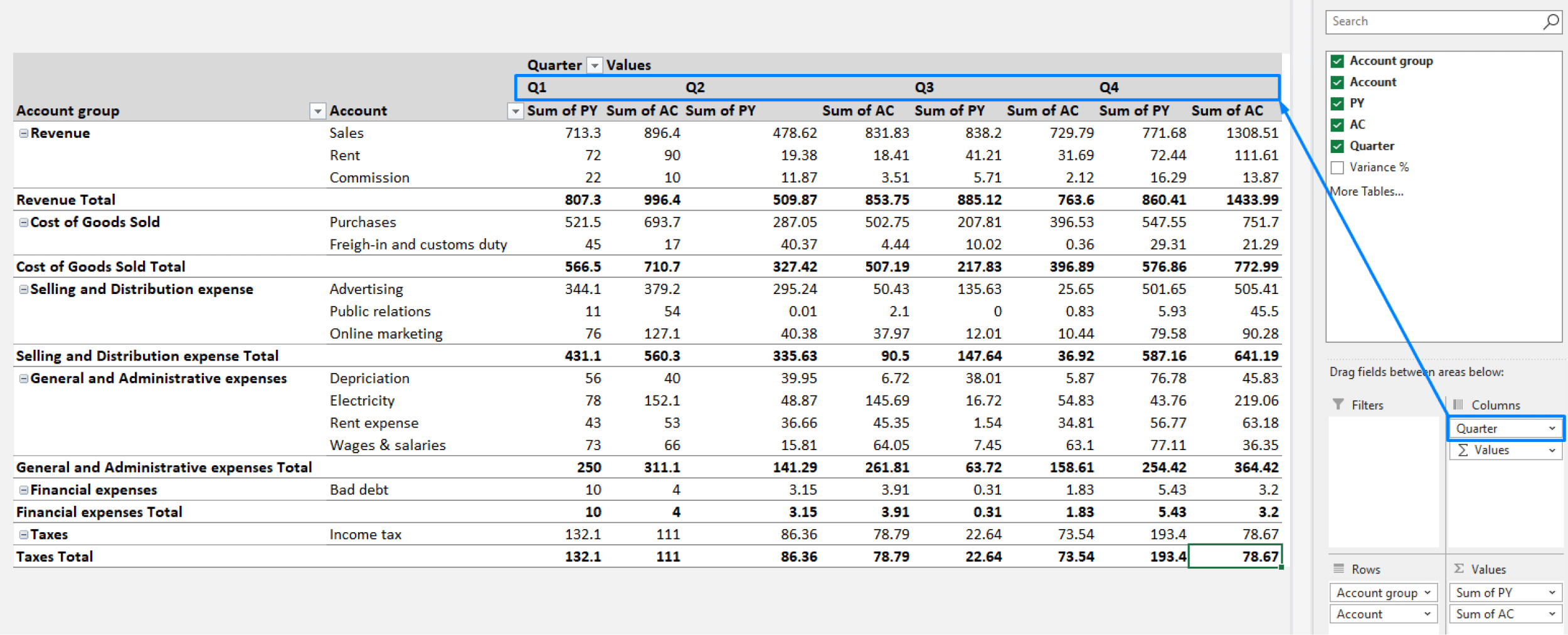
The following resource provides an excellent animated example of grouping data by quarters.
Excel PivotTables | Data Analytics Lesson 14 - Gleim Exam Prep
This article from Gleim Exam Prep includes a clear, animated illustration of date grouping.
Scroll down to the heading "Grouping Datetime Data". First, observe the animation showing the default expand/collapse behavior. Then, pay close attention to the section titled "Example" and its accompanying animation, which shows exactly how to use the Grouping dialog to display results for every quarter, independent of the year.
By mastering this grouping feature, you can slice your data across any time dimension your analysis requires, moving effortlessly from high-level annual summaries to detailed monthly or quarterly reports.
Conclusion
In this lesson, you've moved beyond simple summaries to temporal analysis. You have learned how to leverage Excel's date grouping capabilities to structure your PivotTables for powerful trend analysis.
Key Takeaways:
- Excel automatically groups date fields into a Year > Quarter > Month hierarchy.
- You can Ungroup dates to revert to the raw date list or to apply a new grouping structure.
- The Group dialog box gives you precise control to summarize data by any combination of years, quarters, months, or even days.
- This technique is essential for creating period-over-period financial reports and analyzing trends over time.
In our next lesson, we will make these reports interactive. You will learn how to use Filters and Slicers to dynamically drill down into your summarized data, allowing you to isolate and analyze specific segments like a single product line, region, or salesperson with just a click.