Welcome back! In our previous lesson, we built our first PivotTable, transforming a raw list of transactions into an instant summary. You learned that by default, when you drag a numeric field like 'Amount' into the VALUES area, Excel calculates the SUM. This is a fantastic starting point for totaling revenue or expenses.
Today, we will move beyond this default and take full control over the calculations in our PivotTable. This lesson is all about configuring the value fields to perform different types of summarization. You will learn to switch from SUM to COUNT and AVERAGE, unlocking a much deeper level of analysis. For an accountant, this means being able to answer not just "What was the total revenue?" but also "How many sales did that represent?" and "What was the average value of each sale?"
Beyond the Default: Changing the Calculation
When you create a PivotTable, Excel makes an intelligent guess. If you drop a field with numbers into the VALUES area, it assumes you want to add them up. If you drop a field with text, it assumes you want to count the entries.
The result is that your value field is often named something like "Sum of Sales" or "Sum of Amount".
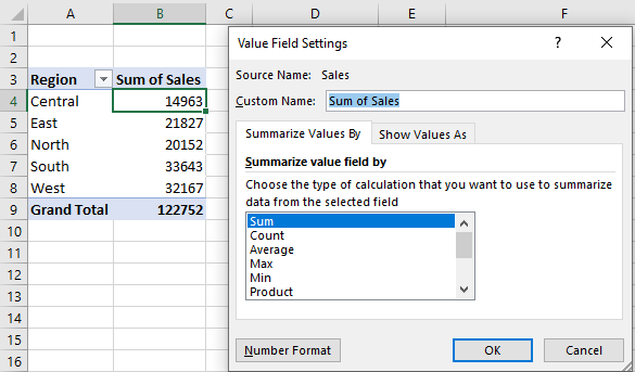
This default is useful, but it's just one of many possibilities. You can easily change this calculation to suit your analysis. The main tool for this is the Value Field Settings dialog box. There are two common ways to access it:
- In the PivotTable Fields pane, left-click the field in the VALUES area and select Value Field Settings.
- Right-click any number inside the values part of your PivotTable. In the context menu, choose Summarize Values By and select an option directly, or click Value Field Settings for more choices.
The following short video demonstrates this second method, which is often the quickest way to adjust your summary.
Pivot Table Excel | Step-by-Step Tutorial
This clip from Kevin Stratvert's tutorial clearly shows how to change the calculation type by right-clicking a value in the PivotTable.
Watch the segment from "summarize the data". Notice how he switches from Sum to Max and then back again. The process is the same for selecting Count or Average.
Once you open the Value Field Settings, you'll see a list of available calculations.

For our purposes as financial analysts, the three most important functions here are:
- Sum: The total of all numbers. Perfect for reporting total revenue, expenses, or assets.
- Count: The number of entries in that field. Crucial for counting transactions, invoices, or employees.
- Average: The arithmetic mean of the numbers. Ideal for finding the average transaction size, average salary, or average days to pay.
Using COUNT for Deeper Insights
Let's put this into a practical accounting context. Imagine you have a list of all sales transactions for the year. A SUM will give you the total revenue. But what if you want to know which month was the busiest in terms of activity, not just revenue? This is where COUNT is essential.
You can change the value field from Sum of Amount to Count of Amount to see the number of transactions per month. A high-revenue month might have been driven by a few large sales, while a month with a high transaction count might indicate strong, broad-based customer activity.
The article from PivotXL provides a simple example of this principle.
Pivot Table Practice Examples in Excel (Free Workbook) - PivotXL
This resource provides concise examples of different PivotTable configurations.
In the "Examples & Solutions" section, review Example 2. This demonstrates setting the Values field to count transaction IDs to find the number of transactions per month.
This concept is directly applicable to many accounting tasks. For instance, in payroll analysis, you wouldn't sum employee ID numbers; you would count them to get a headcount.
The following resource explains this precise application.
MASTERING PIVOT TABLES FOR FINANCIAL ANALYSIS
This article provides real-world applications of PivotTable configurations for financial analysis.
Navigate to the section "2. Headcount and Payroll Analysis" and read the first bullet point, "What is the total headcount by department?". This is a perfect illustration of using Count in a relevant business context.
Using AVERAGE for Performance Metrics
Now let's consider AVERAGE. Continuing our sales analysis, knowing the average sale value is a key performance indicator. If your total revenue is increasing, is it because you're making more sales (higher Count) or because your sales are becoming more valuable (higher Average)? A PivotTable can answer this instantly.
By changing the calculation to AVERAGE, you can quickly create a report showing the average transaction value by region, by salesperson, or over time. This helps identify where your most valuable business is coming from.
The video from Leila Gharani provides another quick walkthrough of changing the calculation, this time to Average.
Excel Pivot Table EXPLAINED in 10 Minutes (Productivity tips included!)
This clip shows how to use the Value Field Settings dialog box to switch a calculation to Average.
Watch the short segment from "go to Value Field Settings".
Again, let's turn to a direct accounting application. When analyzing payroll, the total salary expense (SUM) is important, but the average salary by department or job title (AVERAGE) provides crucial context for budgeting and compensation analysis.
The same article we just viewed has an excellent example of this.
MASTERING PIVOT TABLES FOR FINANCIAL ANALYSIS
Let's return to the same resource for another practical example.
This time, read the second bullet point in the "2. Headcount and Payroll Analysis" section: "What is the average salary by job title?". This shows how changing the calculation to Average can provide powerful analytical insights from the same dataset.
By mastering these three summary calculations—Sum, Count, and Average—you can extract a far greater range of insights from a single dataset, moving from simple reporting to true analysis.
Conclusion
In this lesson, you've learned how to harness the full calculation power of the PivotTable's VALUES area. You are no longer limited to the default SUM and can now tailor your summary reports to answer more sophisticated analytical questions.
Key Takeaways:
- Excel defaults to
SUMfor numeric fields andCOUNTfor text fields in the VALUES area, but this can be changed. - You can change the calculation type by right-clicking a value in the PivotTable and selecting from the Summarize Values By menu, or by using the Value Field Settings.
SUMis for totals (e.g., total revenue).COUNTis for activity volume (e.g., number of invoices).AVERAGEis for key performance indicators (e.g., average sale value).
In our next lesson, we will explore another fundamental PivotTable skill: grouping. You've seen how PivotTables can automatically group dates into years. We will learn how to manually control this grouping to analyze data by months, quarters, and custom date ranges, which is essential for creating trend reports and period-over-period analysis.