Welcome back to our final module on building interactive dashboards. In the last lesson, you installed the "ignition switch" for your dashboard by adding buttons to execute your data refresh and KPI update macros. Your dashboard is now automated, but it's not yet fully interactive.
This lesson is about adding the steering wheel. You will learn how to add a form control dropdown menu that allows a user to dynamically filter the data displayed on the dashboard. For example, a manager could select a specific region or product line from the dropdown, and all the charts and KPIs would instantly update to reflect that choice. This skill is fundamental to creating powerful, self-service business intelligence tools in Excel.
We will accomplish this by:
- Inserting a "Combo Box" form control.
- Linking it to a list of choices and a helper cell.
- Modifying your dashboard formulas to use the selection as a dynamic filter criterion.
Understanding the Combo Box Form Control
The control we'll use is the "Combo Box". It looks like a dropdown list but has a key difference from the data validation lists you've used before. A data validation list lives inside a cell. A combo box is an object that floats on top of the worksheet. This object doesn't hold the selected value itself; instead, it writes a number to a linked cell, representing the user's choice.
The following video from Leila Gharani provides an excellent conceptual overview and demonstrates how to set up the control.
How to make a ComboBox (dropdown) in Excel without VBA
This video clearly explains how the Combo Box works and walks through the crucial setup steps. Pay close attention to the concepts of the "Input Range" and the "Cell Link."
First, watch from the main setup. This section shows you how to insert the Combo Box from the Developer tab and configure its two most important properties in the "Format Control" window.
The Three Key Components
As you saw in the video, making a combo box work involves three distinct parts on your worksheet:
-
The Input Range: This is a list of the items you want to appear in the dropdown. For an accounting dashboard, this could be a list of company divisions, regions, or financial quarters. It's best practice to have this list in a dedicated column, perhaps on a hidden helper sheet.
-
The Combo Box Control: This is the dropdown object itself, which you insert from the
Developer > Insertmenu.
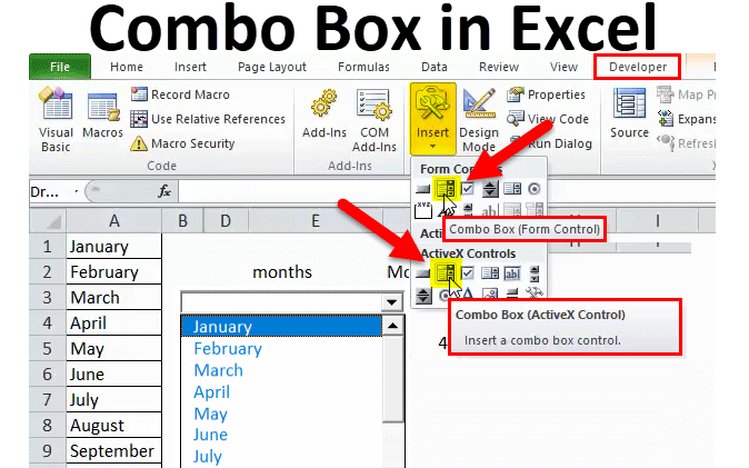
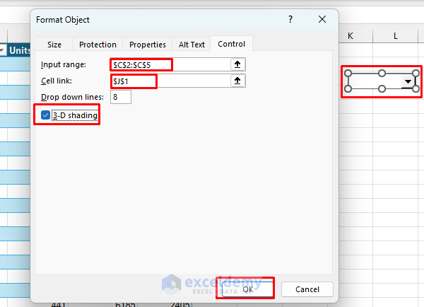
- The Cell Link: This is a single cell that you designate in the "Format Control" settings. When a user selects an item from the dropdown, this cell will display the positional index of that item in the input range (e.g., 1 for the first item, 2 for the second, and so on).
From Index Number to Dynamic Filter
The cell link gives us a number, but our financial formulas (like SUMIFS) need a text criterion, such as the region name "North" or the product category "Services". So, how do we bridge this gap? We use the INDEX function, which you learned about in Module 3.
The INDEX function can take a range of values (our input range) and return a specific value based on its position (our cell link).
The formula is simple: =INDEX(Input_Range, Cell_Link_Value)
Let's see this in action.
How to make a ComboBox (dropdown) in Excel without VBA
The same video demonstrates precisely how to use the INDEX function to solve this problem.
Now, watch from retrieving the name. This clip shows how the INDEX formula is constructed to translate the numeric output from the cell link back into the actual text of the selected month.
Once you have a cell that dynamically displays the selected text (e.g., "North"), you can use it to drive your entire dashboard. You simply point your existing SUMIFS, COUNTIFS, or other reporting formulas to this cell.
For example, a static formula to sum sales for the North region might be:=SUMIFS(Transactions[Amount], Transactions[Region], "North")
Your new, dynamic formula would be:=SUMIFS(Transactions[Amount], Transactions[Region], G1)
...where G1 is the cell containing your INDEX formula.
Now, whenever a user selects a new region from the combo box, the following happens instantly:
- The "Cell Link" cell updates with the new index number.
- The
INDEXformula updates to show the corresponding region name. - The
SUMIFSformula recalculates based on the new region name, updating your dashboard's KPIs and charts.
This entire process of linking controls to dynamic formulas is fundamental to building interactive reports. The following reading provides another example of this workflow.
How to Create Interactive Dashboards with Form Controls ...
This article from Exceldemy provides a great walkthrough of the end-to-end process. While it uses the modern FILTER function, the underlying principle of linking a control to a helper cell and then using that cell in a formula is exactly what we are focusing on.
Focus on Step 2, which shows the insertion and linking of several controls, including a combo box. Then, review the section on dynamic formulas to see how the output of the control is used to drive data filtering.
Your Task: Implement a Dynamic Filter
It's time to apply this to your financial dashboard.
- Decide on a category to filter by (e.g., region, department, product line). On a helper worksheet, create a clean, unique list of the items in that category. This will be your Input Range.
- Navigate to your "Dashboard" worksheet. From the
Developertab, insert a Combo Box (Form Control). - Right-click the new combo box and select "Format Control".
- Set the Input range to the list you created in step 1.
- Set the Cell link to an empty cell on your helper sheet (e.g.,
HelperSheet!A1). Click OK.
- Test the combo box. You should see the items from your list, and when you select one, a number should appear in your cell link.
- In a second cell on your helper sheet (e.g.,
HelperSheet!A2), write anINDEXformula that references your input range and your cell link to retrieve the selected item's text. - Finally, go to your dashboard's calculation area. Modify one of your key
SUMIFSformulas. Instead of a hardcoded text criterion, change it to reference the cell containing yourINDEXformula (HelperSheet!A2). - Return to your dashboard and change the selection in the dropdown menu. You should see the corresponding KPI value update automatically.
Conclusion
You have now added a powerful layer of interactivity to your dashboard. By combining a simple form control with the INDEX function and your existing SUMIFS formulas, you've enabled users to explore the data on their own terms.
Key Takeaways:
- Combo Box (Form Control) is an object that provides a dropdown list for user selection.
- It is configured with an Input Range (the list of choices) and a Cell Link (which outputs the numeric position of the selection).
- The
INDEXfunction is the essential bridge that converts the numeric output of the cell link back into a usable text value. - By linking your dashboard's aggregation formulas (
SUMIFS, etc.) to the output of theINDEXfunction, you make your entire report dynamic.
In our next and final lesson, we will address the last step in the reporting cycle: distribution. You will learn how to write a macro that exports your finished, interactive dashboard to a clean, professional PDF file, ready to be shared with stakeholders.