Welcome to the first lesson of our module on "Data Retrieval and Structuring." In the previous module, we focused on performing calculations within a single dataset, using logical, rounding, and date functions to add intelligence to our spreadsheets. You learned how to manage dates for aging reports, round figures for financial statements, and apply conditional logic with IF.
Now, we shift our focus from calculating new information to retrieving existing information. In any accounting role, your data will rarely exist in one perfect table. You'll have transaction lists, charts of accounts, employee directories, and customer lists, all in separate places. The skill is to link them. This lesson introduces VLOOKUP, one of Excel's most famous functions. It's the digital equivalent of taking an account code, walking over to a large ledger book, and finding the corresponding account name. Mastering this will enable you to merge and enrich datasets, a foundational step in automating financial reports.
The Anatomy of a Vertical Lookup
At its core, VLOOKUP searches for a specific value in the first column of a table and returns a related value from a different column in the same row. The 'V' stands for 'Vertical', as it scans down a column to find your item.
The function has four parts, called arguments, that you must provide:
=VLOOKUP(lookup_value, table_array, col_index_num, [range_lookup])
Let's break this down in an accounting context. Imagine you have a trial balance with account codes (e.g., 6100) and you want to pull in the account names ("Salaries and Wages") from a separate Chart of Accounts table.
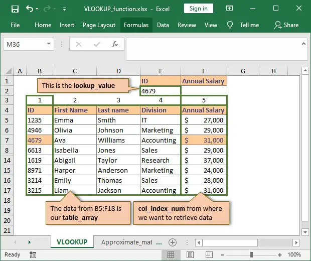
lookup_value: This is the piece of information you already have. It's the unique identifier that links your two tables. In our example, it's the account code6100.table_array: This is the reference table where you want to search for the information. It's your complete Chart of Accounts. A critical rule ofVLOOKUPis that the column containing yourlookup_value(the account codes) must be the first column of this table array.col_index_num: This is the column number in your table array from which you want to retrieve a value. If your Chart of Accounts has account codes in column 1 and account names in column 2, you would enter2to get the name.[range_lookup]: This is an optional but crucial argument. It can beTRUEorFALSE.FALSE: This tells Excel to find an exact match. For accounting tasks like matching account codes, invoice numbers, or employee IDs, this is what you will use 99% of the time. If an exact match isn't found, Excel will return an error.TRUE: This tells Excel to find an approximate match. It's used for finding values within a range, like tax brackets or commission tiers. We will touch on this later, but for now, focus onFALSE.
The Corporate Finance Institute has a clear article that defines these arguments.
VLOOKUP - Corporate Finance Institute
This guide provides a clear, textual breakdown of the VLOOKUP function and its arguments.
Please read the sections VLOOKUP Formula and the subsequent numbered list that details each argument. This will solidify your understanding of the four key components.
The image below provides a great visual breakdown of how these arguments fit together in a real formula.
VLOOKUP in Action: Populating a Chart of Accounts
Let's apply this to the most common accounting use case: matching account descriptions to account codes. In the following video, Leila Gharani provides a concise demonstration. Pay close attention to how she defines each of the four arguments, especially her emphasis on using FALSE for an exact match and using the F4 key to make the table_array an absolute reference—a key concept from our first module.
Excel for Accounting - 10 Excel Functions You NEED to KNOW!
This clip from Leila Gharani's "Excel for Accounting" series demonstrates the classic use of VLOOKUP to enrich a list of transactions with data from a lookup table.
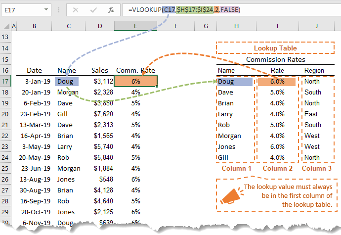
Watch the segment from the beginning of the VLOOKUP section. Notice how the lookup value (account number) is in the first column of the lookup table. This is a strict requirement for the function to work.
The image below reinforces this critical rule. The lookup_value (the salesperson's name) must be in the first column of the lookup table. The function cannot look to its left.
A Practical Walkthrough and a Best Practice
Now, let's watch a more detailed, step-by-step example. In this video, Hector Garcia, a CPA, demonstrates how to use VLOOKUP to pull payee names into a bank transaction list. He also introduces an important best practice: formatting your lookup range as an official Excel Table (Ctrl+T). When you do this, you can refer to the table by name instead of a cell range (e.g., Table1 instead of $H$17:$J$24). This makes your formulas easier to read and automatically adjusts if you add more data to your lookup table.
How to use VLOOKUP in Excel for Accounting
This video from Hector Garcia CPA provides a detailed, practical demonstration of using VLOOKUP to reconcile accounting data.
Watch this segment from the main VLOOKUP demonstration. Focus on two key moments: His process of thinking through the formula: what he's looking for, where he's looking, and what he wants back. His use of Ctrl+T to create a named table (Table1). Notice how this simplifies the table_array argument in his formula.
Troubleshooting: When VLOOKUP Fails
Sometimes, VLOOKUP returns an #N/A error, which means "Not Available." This happens when Excel cannot find your lookup_value in the first column of the table_array.
advanced excel – vlookup, hlookup and pivot tables
This guide from Carnegie Mellon University provides a very detailed look at VLOOKUP, including how to interpret and resolve common errors.
Read the section that begins after the formula is copied down, starting from the explanation of #N/A. The document then walks through how to fix it by adding the missing data to the source table.
One of the most common and frustrating reasons for an #N/A error is hidden extra spaces in your cells. Data exported from accounting systems or copied from other sources can often have leading or trailing spaces (e.g., " 1100" instead of "1100"). To VLOOKUP, these are not the same value.
The solution is to wrap your lookup_value inside the TRIM function, which removes these extra spaces.
=VLOOKUP(TRIM(A2), ChartOfAccounts, 2, FALSE)
Leila Gharani demonstrates this exact scenario and its solution beautifully.
Excel for Accounting - 10 Excel Functions You NEED to KNOW!
This is a continuation of the previous video. It addresses a very common real-world problem when using lookup functions.
Now watch the next section on the TRIM function from this timestamp. See how her VLOOKUP initially fails and how nesting the lookup_value inside TRIM instantly solves the problem. This is a vital technique for data cleaning.
A Note on Approximate Match (TRUE)
While FALSE is your default for most accounting tasks, VLOOKUP can also perform an approximate match. This is useful for tiered calculations, like finding a tax rate or a commission percentage based on a sales amount. For this to work, the first column of your table_array must be sorted in ascending order.
The function will scan down the list and stop at the largest value that is less than or equal to your lookup_value. For instance, if you have tiers at $0, $100, and $1000, and your lookup value is $500, it will match with the $100 tier.
For a demonstration, you can watch this part of Hector Garcia's video where he uses an approximate match to categorize transactions as 'low', 'medium', or 'high' value.
How to use VLOOKUP in Excel for Accounting
This final clip from Hector Garcia's video explains the use case for the 'TRUE' or approximate match argument in VLOOKUP.
Watch this segment from where he discusses approximate match. Observe how he builds a small table with value tiers and uses VLOOKUP with the TRUE argument to classify each transaction.
Conclusion
In this lesson, you have learned how to use the VLOOKUP function to retrieve data from vertical tables. This is a fundamental skill for connecting disparate accounting datasets, such as bringing account names into a transaction list.
Key Takeaways:
VLOOKUPhas four arguments:lookup_value,table_array,col_index_num, andrange_lookup.- The
lookup_valuemust be in the first column of thetable_array. - For accounting reconciliations, always use
FALSEfor an exact match. - The
#N/Aerror means a match was not found. Use theTRIMfunction to eliminate hidden spaces, a common cause of this error. - Use absolute references (
$A$1:$B$10) or named Excel Tables for yourtable_arrayto prevent errors when copying formulas.
VLOOKUP is powerful, but it has limitations. It can only look to the right, and inserting columns can break the col_index_num. In our next lesson, we will explore a more flexible and robust alternative: using the INDEX and MATCH functions together. This combination overcomes VLOOKUP's weaknesses and is the preferred method for many Excel professionals.