Welcome back. In our last two lessons, we systematically built a dynamic Income Statement and a dynamic Balance Sheet, pulling data directly from a trial balance using SUMIFS and a mapping table. You now have the core components of an automated financial reporting model.
Today, we shift our focus from construction to validation. A financial model is only useful if it's accurate, and the most fundamental rule of accounting—the accounting equation—provides a perfect opportunity to build an automated safety net. Our goal is to create a check formula that continuously verifies that your Balance Sheet balances. This is not just a best practice; it is an essential feature for any reliable financial model.
The Principle of a Balance Check
Your accounting education provides the foundational knowledge here: the Balance Sheet must always balance.
Assets = Liabilities + Equity
Therefore, it logically follows that:
Assets - Liabilities - Equity = 0
Our task is to translate this fundamental equation into a live formula within our Excel model. This formula will act as a constant guard, immediately alerting us if any action—a data update, a formula change, or an incorrect mapping—causes the Balance Sheet to become unbalanced.
A simple, effective way to implement this is to create a formula that calculates this difference. If the model is correct, the result is zero. If not, the result is the exact amount of the discrepancy, which can be a powerful clue for debugging.
The resource below explains this approach and shows how you can use conditional formatting to make any error impossible to miss.
Error Checks For Excel And Financial Modelling | Model Citizn
This article from Model Citizn discusses various error-checking techniques in financial modeling.
Please read the section that begins with the image of a #DIV/0! error. Focus on the part titled The Balance Sheet Check, and study the simple but effective formula provided: =IF((C3-C5-C7)<>0, (C3-C5-C7),0). This formula checks if the difference is not zero, and if so, it displays the difference.
The image below, taken from the article, illustrates this perfectly. In the "NO BS ERROR" scenario, the check cell is zero. In the "BS ERROR" scenario, the formula immediately flags the (22) discrepancy.

Building a More Robust Check System
While displaying the error amount is useful for investigation, for summary dashboards and high-level reporting, it's often better to create a binary "flag" system: 0 for "OK" and 1 for "Error". This allows you to easily sum or count all the errors in your model.
This concept is part of a more systematic approach to model validation, which is explored in detail in the following article from Financial Management magazine.
Excel modelling: How to implement 3 types of checks
This article provides a comprehensive guide to building robust check mechanisms in Excel, using a Balance Sheet check as the primary example.
First, read the introduction to understand the different types of checks. Next, see how a simple check is developed in the section with the heading Simple Balance Sheet with Check. Notice the author's critique of using a simple TRUE/FALSE output and the introduction of the *1 technique to convert it to 1/0. Now, read the section on refining the formula. This is a crucial step. Pay close attention to the explanation of why the ROUND function is necessary to handle Excel's minor floating-point inaccuracies. Continue to the section on adding a prima facie check. This addresses what happens if a cell reference is deleted, causing an error like #REF!. Using ISERROR to catch this before performing the balance check makes your model much more resilient. Finally, review how to aggregate checks across multiple time periods into a single summary dashboard. The use of MAX is a particularly elegant way to create a master error flag.
Deconstructing the Robust Check Formula
Let's consolidate the key steps from the article to build our best-practice check system. We will create two separate checks for clarity and robustness.
Assume Total_Assets is in cell C12, Total_Liabilities is in C18, and Total_Equity is in C20, matching the layout of a standard Balance Sheet.
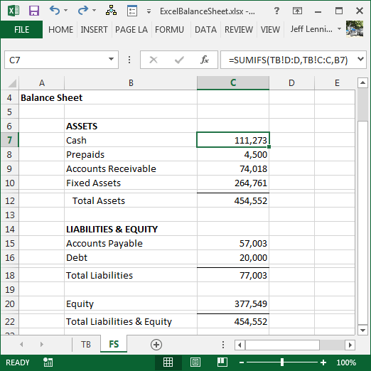
Step 1: The "Prima Facie" Error Check
This check doesn't test the balance; it tests if the numbers can even be calculated. It looks for errors like #REF!, #VALUE!, or #DIV/0! in your core totals.
The formula would be:=IF(ISERROR(C12-C18-C20), 1, 0)
ISERROR(...)returnsTRUEif the calculation inside results in any error.- The
IFstatement converts thisTRUE/FALSEinto a1(Error) or0(OK).
Step 2: The Balance Check (with Rounding)
This second check performs the actual accounting validation, but only if the first check passed. It also uses ROUND to prevent false alarms from insignificant floating-point discrepancies.
The formula would be:=IF(check_cell_from_step_1 = 1, 0, (ROUND(C12-C18-C20, 2) <> 0) * 1)
Let's break this down:
IF(check_cell_from_step_1 = 1, 0, ...): If the prima facie check found an error, this formula returns0to avoid double-counting the error.... ROUND(C12-C18-C20, 2): We calculate the difference and round it to 2 decimal places (standard for currency).... <> 0: We check if this rounded difference is not equal to zero. This returnsTRUEorFALSE.... * 1: This converts theTRUE(an error exists) to1andFALSE(all is well) to0.
Step 3: The Aggregator Check
If your model spans multiple periods (e.g., Jan, Feb, Mar), you'll have a set of these checks for each month. To create a single master error light on a summary page, you can use the MAX function.
=MAX(range_of_all_check_cells)
Since our check cells only contain 0 or 1, the MAX function will return 1 if even a single error exists anywhere in the range, and 0 only if everything is perfect. This is an incredibly efficient way to monitor the health of your entire model at a glance.
Conclusion
You have now added a critical layer of integrity to your financial model. By automating the verification of the fundamental accounting equation, you build confidence in your reports and create a system that flags errors the moment they occur.
Key Takeaways:
- A Balance Sheet check (
Assets - Liabilities - Equity = 0) is a non-negotiable component of any financial model. - A simple check can show the magnitude of the error, which aids in debugging.
- A robust check system uses binary flags (
0for OK,1for Error) and proactively handles potential issues like floating-point discrepancies (ROUND) and precedent formula errors (ISERROR). - Aggregator functions like
MAXare used to consolidate individual checks into a single master error flag for high-level dashboards.
With your dynamic Income Statement and Balance Sheet now built and validated, you are ready to use them for analysis. In our next lesson, we will leverage these statements to calculate key profitability and liquidity ratios, turning your automated reports into powerful tools for business insight.