Time Value of Money: Discounting, Compounding, and Growth Assumptions

Introduction

In the last module, you became a financial detective, learning to tear apart a company's past performance by dissecting its financial statements and, more importantly, reading the fine print in the annual report. You now know how to assess what a company has done. Today, we pivot from forensics to forecasting. We move from analyzing the past to valuing the future.

This lesson introduces the single most important concept in finance: the Time Value of Money (TVM). It's the engine that powers every valuation model. We will master the mechanics of compounding and discounting, the tools used to move cash flows across time. More critically, you will see how these tools are applied to value a stock and, in doing so, discover how wildly a company's perceived worth can swing based on a few key assumptions about its future growth. This is where the abstract art of storytelling meets the hard science of numbers, and it's the foundation for developing the "scary accuracy" you're aiming for.

The Financial Engine: Compounding and Discounting

At its heart, the time value of money is built on a simple, powerful idea: a rupee today is worth more than a rupee tomorrow. This isn't a philosophical statement; it's a financial reality driven by two factors:

Opportunity Cost: A rupee today can be invested to earn a return, becoming more than a rupee tomorrow.
Risk: The future is uncertain. A promised rupee tomorrow might never arrive.

These two ideas give rise to two fundamental operations: compounding and discounting.

This image illustrates the symmetrical relationship between compounding money forward into the future and discounting it back to the present.

Compounding: Calculating Future Value (FV)

Compounding is the process of determining the future value of a present sum of money. If you invest ₹100 today at a 5% annual interest rate, in one year you'll have ₹105. The next year, you earn 5% on the entire ₹105, not just the original ₹100. This process of earning a return on your returns is the essence of compounding.

The formula is:

F V = P V \times (1 + r)^{n}

Where:

$F V$ = Future Value
$P V$ = Present Value (your initial amount)
$r$ = The interest rate per period
$n$ = The number of periods

For your IT background, you can think of this as an iterative loop where the value at the end of each period becomes the input for the next, accumulating exponentially.

Discounting: Calculating Present Value (PV)

Discounting is the reverse of compounding and is the absolute bedrock of valuation. It answers the crucial question: "What is a promise of future cash worth to me today?"

To find the present value, we simply rearrange the FV formula:

P V = \frac{F V}{( 1 + r ) ^{n}}

Here, r is called the discount rate. It represents the rate of return you require to justify waiting for the future cash flow and taking the associated risk. A higher discount rate means you are less willing to wait or perceive more risk, so you value the future cash flow less today. A lower discount rate implies the opposite.

As the image shows, discounting a future amount of ₹127.6 back over 5 periods at a 5% rate returns it to its present value of ₹100. Every valuation you will ever perform is, in essence, an application of this single concept.

Applying TVM: From Theory to Stock Valuation

A stock is not just a ticker symbol; it's a claim on a company's future cash flows. Therefore, the intrinsic value of a stock is the present value of all the cash flows an investor expects to receive from it.

The most straightforward model to demonstrate this is the Dividend Discount Model (DDM). It assumes the cash flows an investor receives are the company's dividends.

Stock Valuation

This video, "Stock Valuation" from the channel Fresh Finance with Professor McElfresh, provides a clear, step-by-step introduction to the DDM. It will walk us through the logic of how we can value a stock by making different assumptions about its future dividend growth.

First, watch the introduction from the beginning to understand why valuing stocks is harder than valuing bonds and how the price is defined as the present value of future dividends. Next, watch the segment on the simplest assumption, zero growth. This treats the stock like a perpetuity, a stream of constant cash flows forever. The formula is simply P_0 = D/r. Now for the most important part. Watch the explanation of the constant growth model, also known as the Gordon Growth Model. This is a true workhorse of valuation. Pay close attention to the formula: P_0 = \frac{D_1}{r - g} Notice two critical things: The numerator is D_1, the dividend one year from now, not the dividend that was just paid (D_0). The denominator is r - g, the difference between the required rate of return and the constant growth rate. This small denominator is a powerful lever.

The power of this model lies in its sensitivity. The value $P_{0}$ is not just a function of the dividend, but is dramatically influenced by your assumptions for r and g. If r is 10% and g is 5%, the denominator is 0.05. If you change your growth assumption to 7%, the denominator becomes 0.03, and the resulting valuation increases by 67%! A small change in the growth assumption leads to a massive change in the output value. This is how two analysts looking at the same company can arrive at wildly different valuations.

The Operator's View: Growth, Rates, and Market Reality

The DDM is a great teaching tool, but professionals typically use a more robust model called the Discounted Cash Flow (DCF) model. It discounts the company's free cash flows (the cash generated by the business available to all investors) rather than just dividends. However, the core engine—discounting future cash flows using r and g—is identical.

The real game is not in building the most complex spreadsheet, but in having the most intelligent assumptions for r and g.

The Discount Rate (`r`) in the Real World

Where does r come from? It's not an abstract number. It's determined by the available alternatives. The safest alternative is usually a government bond.

Interest Rate Effects on Equities: Valuation Impacts - Lyn Alden

This article by Lyn Alden is a masterclass in connecting valuation theory to market dynamics. It explains how interest rates are the gravity of financial markets and affect different types of stocks in different ways.

First, read the introduction, The Equity Risk Premium. This explains that your required return (r) is essentially the risk-free rate (like a government bond yield) plus an "equity risk premium" you demand for taking on the extra risk of owning stocks. Now, read the sections that provide concrete DCF examples for three types of companies, starting from this point. Focus on the key takeaway: a 4% drop in the discount rate (from 12% to 8%) increases the value of a... Value Stock by 44.7% Growth Stock by 61.8% Hypergrowth Stock by 89.9% This is a profoundly important insight. Companies whose value is tied to cash flows far in the future (growth stocks) are far more sensitive to changes in the discount rate than stable companies whose cash flows are more front-loaded (value stocks). This is why rising interest rates (which push discount rates up) have been so brutal for technology and other growth stocks. The Growth Rate (g): Not All Growth is Good Your growth assumption is arguably the most powerful input in a valuation model. But simply projecting high growth is amateurish. A professional asks: is this quality growth?

This is a profoundly important insight. Companies whose value is tied to cash flows far in the future (growth stocks) are far more sensitive to changes in the discount rate than stable companies whose cash flows are more front-loaded (value stocks). This is why rising interest rates (which push discount rates up) have been so brutal for technology and other growth stocks.

The Growth Rate (`g`): Not All Growth is Good

Your growth assumption is arguably the most powerful input in a valuation model. But simply projecting high growth is amateurish. A professional asks: is this quality growth?

[PDF] PRICE AND VALUE: DISCERNING THE DIFFERENCE - NYU Stern

This document from valuation expert Aswath Damodaran gets to the heart of what drives intrinsic value. It separates noise from signal.

Read the section on Expected Growth. Damodaran makes a crucial point: "You can grow while destroying value at the same time." Quality growth only happens when the return on capital (ROC) is greater than the cost of capital (your discount rate). If a company has to invest ₹100 to generate ₹5 of annual profit, while its cost of capital is 8%, that growth is actually making the owners poorer. Skim the valuation example for Twitter. You don't need to follow every number, but look at the key assumptions listed: "Revenue growth of 51.5% a year," "Pre-tax operating margin increases to 25%," "Sales to capital ratio of 1.50." These assumptions are the heart of the model. Change them, and the final valuation of "$17.84/share" changes dramatically.

The Analyst's Reality Check: Sensitivity Analysis

Because valuation is so sensitive to these assumptions, professionals never rely on a single number. They analyze how the valuation changes as the key inputs change. This is called Sensitivity Analysis.

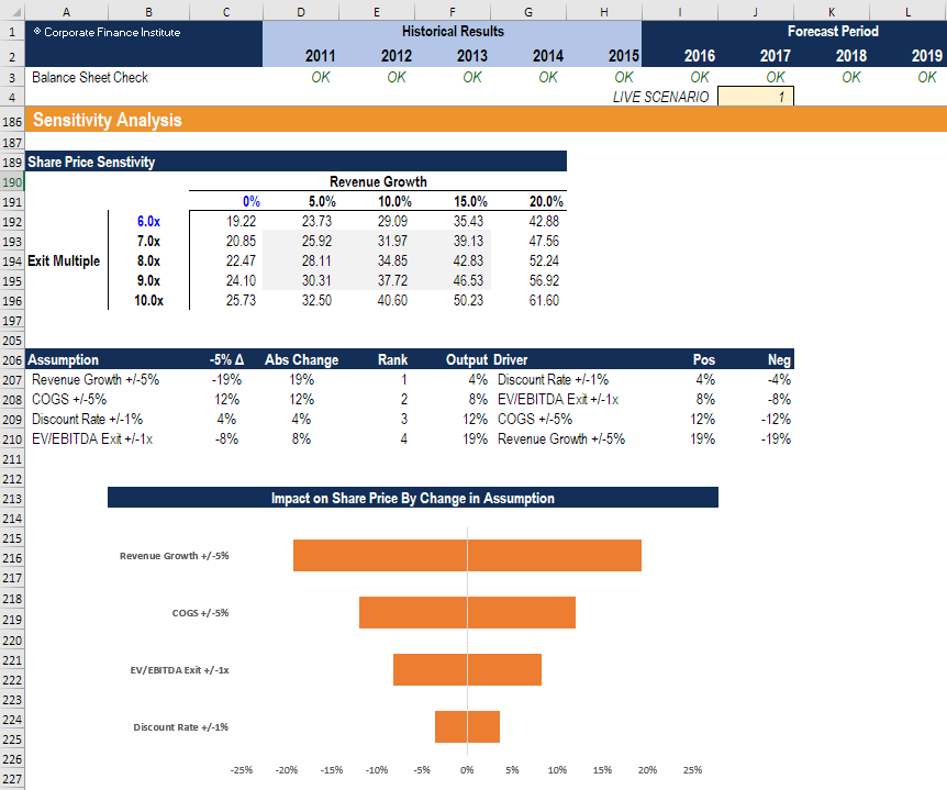
A sensitivity analysis in a financial model. The Tornado Chart on the bottom visually ranks which assumptions have the biggest impact on the output (in this case, Share Price). Notice how Revenue Growth and Exit Multiple (which is a proxy for long-term growth) are the most significant drivers.

This chart is the perfect visual summary of our lesson. It demonstrates that the final valuation is a direct product of the assumptions you make. The operator's edge comes from having a more defensible set of assumptions than the market consensus.

Conclusion

You have now mastered the fundamental mechanics of valuation. You understand that compounding and discounting are the tools we use to translate the promise of future cash into a concrete value today. More importantly, you've seen that valuation is not a black box; it's a model driven by assumptions, and the output is exquisitely sensitive to those inputs.

Key Takeaways:

Time Value of Money (TVM): The core principle that a rupee today is worth more than a rupee tomorrow. Compounding calculates future value; discounting calculates present value.
Valuation as Discounting: The value of any asset is the present value of its expected future cash flows.
The Levers of Value: A stock's valuation is highly sensitive to the discount rate (r) and the growth rate (g).
Growth Stock Sensitivity: Companies with cash flows weighted far in the future (growth stocks) are much more sensitive to changes in r and g than mature, stable companies.
Quality Over Quantity: High growth is only valuable if the return on investment exceeds the cost of capital. Growth can destroy value.

In this lesson, we explored the principle of discounting and saw how sensitive it is to our assumptions. In the next lesson, we will get our hands dirty and start building the analyst's primary tool from the ground up: the Discounted Cash Flow (DCF) model.

Recommended resources