Efficient Hessian-vector Products with JVP and Grad

1. The "Why": Applications of Hessian-Vector Products

Before diving into the "how," let's briefly touch on the "why." Why is the operation $v\mapsto H_f(\theta )v$, the product of the Hessian matrix $H_f(\theta )$ with a vector $v$, so important? In many cases, it's all the information we need.

• Second-Order Optimization: Methods like the Newton-Conjugate Gradient algorithm aim to find an update direction by solving the linear system $H_f(\theta )\Delta \theta =-\nabla f(\theta )$. Iterative solvers for this system, such as the conjugate gradient method, only require the ability to compute products of the Hessian with arbitrary vectors—they never need the full matrix.
• Curvature Analysis: The Hessian's eigenvalues describe the curvature of the loss landscape. Algorithms like the Lanczos method can approximate the dominant eigenvalues and eigenvectors of the Hessian using only HVP computations. This is invaluable for understanding properties like sharpness/flatness of minima, which relates to generalization.

The following blog post provides an excellent overview of these applications.

The key takeaway is that we can unlock the power of second-order information without paying the prohibitive cost of materializing the full Hessian, if we can compute HVPs efficiently.

2. The "How": HVP as a Directional Derivative of the Gradient

The efficient computation of HVPs is based on a crucial mathematical insight, famously articulated by Barak Pearlmutter in 1994. The Hessian-vector product is equivalent to the directional derivative of the gradient function.

Let's break this down.

1. We have a scalar-valued function $f:{\mathbb{R}}^n\to \mathbb{R}$, like a loss function.
2. Its gradient, $\nabla f$, is a function that maps from the parameter space to the gradient space, $\nabla f:{\mathbb{R}}^n\to {\mathbb{R}}^n$.
3. The Hessian, $H_f$, is the Jacobian of the gradient function, $H_f=J_{(\nabla f)}$.
4. The Hessian-vector product, $H_f(x)v$, is therefore the Jacobian of the gradient function multiplied by the vector $v$: $J_{(\nabla f)}(x)v$.

This is precisely the definition of a Jacobian-vector product (JVP) that we've already studied! Specifically, the HVP is the JVP of the gradient function $\nabla f$.

This identity provides a clear recipe for implementation in JAX:

1. Obtain the gradient function using reverse-mode AD (jax.grad).
2. Compute the JVP of that gradient function using forward-mode AD (jax.jvp).

This "forward-over-reverse" approach is the most direct and generally most efficient way to compute an HVP.

3. Implementing HVPs by Composition

Let's translate this insight into code. JAX's compositional nature makes this incredibly straightforward. We will explore the three primary ways to compose differentiation transforms to compute an HVP.

Method 1: Forward-over-Reverse (Recommended)

This method is the direct implementation of the logic we just derived.

import jax
import jax.numpy as jnp

def hvp_forward_over_reverse(f, primals, tangents):



  # f: the function R^n -> R
  # primals: the point x at which to compute the HVP
  # tangents: the vector v to multiply the Hessian by
  



  # The JVP of the gradient function of f.
  # jax.jvp(g, (x,), (v,)) returns (g(x), J_g(x)v)
  # We want the second element.
  return jax.jvp(jax.grad(f), (primals,), (tangents,))[1]

This is elegant and efficient. It involves one reverse-mode pass (for the inner grad) and one forward-mode pass (for the outer jvp). As jvp has a lower memory overhead than a reverse-mode pass, this is a very memory-friendly approach.

The JAX documentation's "Autodiff Cookbook" formalizes this exact method.

Method 2: Reverse-over-Reverse

Another way to think about the HVP is to first define a new scalar-valued function $h(x)=\nabla f(x)\cdot v$, where $v$ is treated as a constant vector. The gradient of this new function, $\nabla h(x)$, is precisely the HVP we want.

Since this involves two gradient operations, we can implement it by nesting jax.grad.

def hvp_reverse_over_reverse(f, primals, tangents):



  # Define the intermediate scalar-valued function.
  # Note: tangents (v) are closed over by the lambda.
  h = lambda x: jnp.vdot(jax.grad(f)(x), tangents)
  



  # The gradient of this function is the HVP.
  return jax.grad(h)(primals)

This approach performs two full reverse-mode passes. As reverse-mode AD requires storing intermediate values from a forward pass for the backward pass, nesting them (grad of grad) can lead to significantly higher memory consumption compared to the forward-over-reverse method.

Method 3: Reverse-over-Forward

Finally, we could flip the first approach. We can define a function that computes the JVP of the original function $f$, which gives the directional derivative ${\nabla }_{v}f(x)$. We can then take the gradient of that result with respect to the original parameters $x$.

def hvp_reverse_over_forward(f, primals, tangents):



  # Define a function that computes the directional derivative.
  jvp_fn = lambda x: jax.jvp(f, (x,), (tangents,))[1]




  # The gradient of the directional derivative is the HVP.
  return jax.grad(jvp_fn)(primals)

This also involves one forward and one reverse pass, and its performance is generally similar to the forward-over-reverse method. However, the ICLR blog post you read earlier notes a practical advantage of forward-over-reverse: it naturally computes the gradient $\nabla f(x)$ as an intermediate value, which can be useful since many optimization algorithms need both the gradient and the HVP.

The following video provides a quick summary of how these higher-order derivatives can be formed by composition.

4. Performance in Practice: The Power of JIT Compilation

We have three methods, and a theoretical reason to prefer forward-over-reverse for memory efficiency. Let's see what happens in practice when running on real deep learning models. The ICLR blog post provides excellent benchmarks.

Let's analyze the results for JAX from that article.

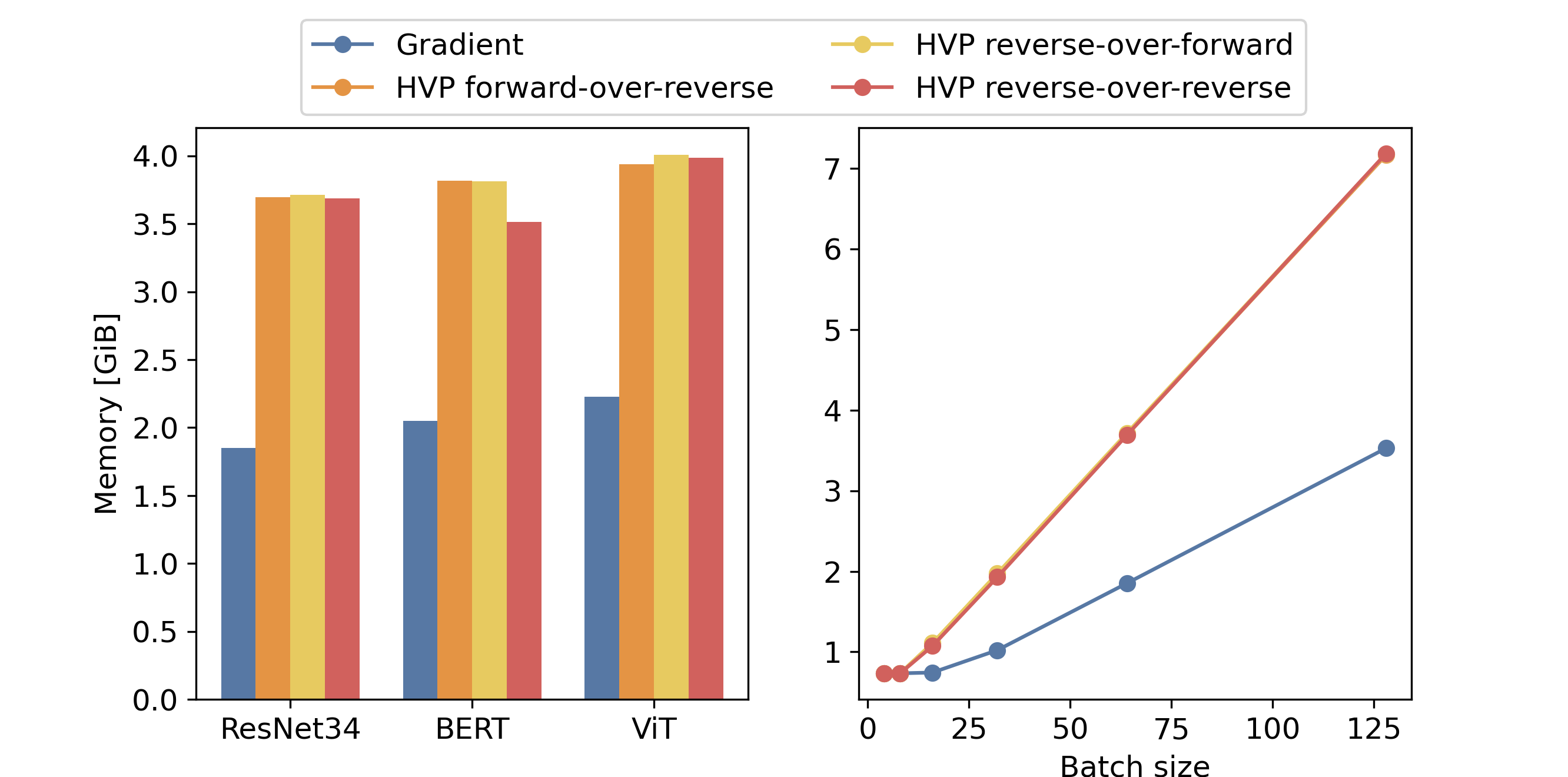
Here are the key observations, which speak volumes about JAX's design:

• Time Complexity: With JIT compilation, all three methods are very close in performance. The total time for an HVP is roughly 2-3 times that of a single gradient computation, which is consistent with the theory (e.g., one forward pass + one reverse pass).
• Memory Complexity (with JIT): The most surprising result is on the left plot. The memory usage for all three methods is nearly identical! This seems to contradict our theory that reverse-over-reverse should be more memory-hungry. The article correctly points out that this is due to XLA's powerful fusion and memory optimization capabilities. The JIT compiler is smart enough to analyze the entire computation graph and optimize memory allocation, largely erasing the theoretical differences between the methods when compiled.
• Memory Complexity (without JIT): The authors perform a crucial experiment: disabling JIT. In that case, the results match theory perfectly—reverse-over-reverse consumes significantly more memory. This is a fantastic illustration of the value added by the compiler.

Your interest in JAX's internals and compilation makes this a particularly important point. The high-level functional transformations define the what (compute an HVP), but the JIT compiler (XLA) has significant freedom in determining the how (the specific, fused execution kernel), often leading to performance characteristics that are better than what a naive analysis of the uncompiled code would suggest.

Conclusion

In this lesson, we demystified the Hessian-vector product, a cornerstone of many advanced machine learning techniques. You now have the tools to compute second-order derivatives efficiently at any scale.

Key Takeaways:

• Hessian-vector products (HVPs) allow us to leverage second-order derivative information without the prohibitive cost of materializing the full Hessian matrix.
• The most efficient HVP implementations are based on the identity $H_f(x)v=J_{(\nabla f)}(x)v$, which frames the HVP as the JVP of the gradient function.
• In JAX, this is implemented by composing jvp and grad. The forward-over-reverse method, jax.jvp(jax.grad(f), ...), is generally recommended as it is conceptually direct and memory-efficient.
• While other compositions like reverse-over-reverse exist, they are theoretically less memory-efficient. However, JAX's JIT compiler (XLA) can often optimize these differences away, showcasing the power of compilation in high-performance computing.

In our next lesson, we will venture further into the customization of JAX's differentiation engine. You will learn how to define custom differentiation rules for your functions using jax.custom_vjp, giving you complete control over the backward pass. This is an advanced technique essential for implementing novel algorithms or for manually optimizing gradient flow in complex models.