Hello! Welcome to the next lesson in our exploration of JAX's automatic differentiation system.
In our last session, we saw how to compose JAX's high-level differentiation primitives, grad and jvp, to construct powerful second-order operations like Hessian-vector products. We treated JAX's autodiff as a mostly black box, trusting it to correctly derive and execute the backward pass. Today, we're going to open that box.
This lesson addresses a key question for anyone implementing novel algorithms or pushing performance limits: What happens when the default gradient computed by the system isn't what you want? You will learn how to take full control of the backward pass by defining a custom vector-Jacobian product (VJP) rule for any function using jax.custom_vjp. This powerful technique is essential for improving numerical stability, optimizing performance, and defining gradients for non-differentiable functions.
1. Backpropagation as a Chain of Vector-Jacobian Products
Before diving into the JAX API, it's crucial to solidify the mathematical foundation. As you know from your extensive deep learning experience, training neural networks relies on backpropagation, which is a specific, highly efficient implementation of reverse-mode automatic differentiation.
The core operation at each step of the backward pass is the vector-Jacobian product (VJP). For a function and a scalar loss that depends on , the chain rule gives us the gradient of the loss with respect to the input :
Here, is the "upstream gradient" (or cotangent vector) coming from later stages of the computation. The VJP is the operation that takes this upstream gradient and produces the "local gradient" . Backpropagation is simply a chain of these VJP calculations, propagating the gradient from the final loss all the way back to the input parameters.
The following article provides an excellent mathematical treatment of this concept, which should resonate with your background.
Everything You Need to Know About Backpropagation | George Assaad
This article by George Assaad provides a rigorous yet clear explanation of backpropagation from first principles. It's a perfect refresher on the mathematics that underpins JAX's grad and vjp transformations.
Please read the first two sections, "The Core Theory of Backpropagation" and "Forward vs. Reverse Mode: Why Backprop Wins". As you read, focus on the definition of the VJP and how the article illustrates the computational cost difference between forward and reverse modes. This cost analysis is the fundamental reason why deep learning frameworks are built on reverse-mode AD.
2. The VJP "Trick": Never Materialize the Jacobian
The most critical insight for efficient backpropagation is that we almost never explicitly form the full Jacobian matrix . For a typical neural network layer, this matrix can be enormous. Instead, we implement a function that directly computes the result of multiplying its transpose by the upstream gradient vector.
This "VJP trick" is the key to both performance and memory efficiency. By deriving an analytical expression for , we can bypass the costly matrix formation entirely. The article you just started provides a fantastic derivation for a linear layer.
Everything You Need to Know About Backpropagation | George Assaad
This section continues the theoretical discussion with a concrete example.
Now, please read the section "The VJP Trick: Never Materialize Jacobians", including the derivation for a linear layer. Pay close attention to how the complex expression involving a large, sparse Jacobian simplifies into a simple outer product: \nabla_W \mathcal{L} = (\nabla_y \mathcal{L}) \cdot x^T. This is the analytical "shortcut" we will implement.
This simplification is profound. The backward pass for a linear layer doesn't require a massive matrix-vector product, but rather a much cheaper outer product between two vectors: the upstream gradient and the input vector from the forward pass. This is precisely the kind of optimization we can enforce using a custom VJP.
3. Implementing jax.custom_vjp
JAX provides the @jax.custom_vjp decorator to allow you to specify your own backward pass. This is analogous to torch.autograd.Function in PyTorch.
Using it involves three steps:
- Decorate your main function (e.g.,
Linear) with@jax.custom_vjp. This function defines the forward computation as usual. - Define a forward rule (
_fwd). This function takes the same inputs as your main function. It must return a tuple containing:- The result of the forward pass (the same as the main function).
- A
residualstuple, containing any intermediate values from the forward pass that are needed for the backward pass.
- Define a backward rule (
_bwd). This function takes two arguments:- The
residualstuple saved by the forward rule. - The upstream gradient
g(i.e., ).
It must return a tuple of gradients corresponding to each input of the main function.
- The
- Link the rules to the main function using
my_function.defvjp(my_function_fwd, my_function_bwd).
Let's look at the computational graph for a Vector-Jacobian Product. The backward pass, which is what we are customizing, traces the computation in reverse.
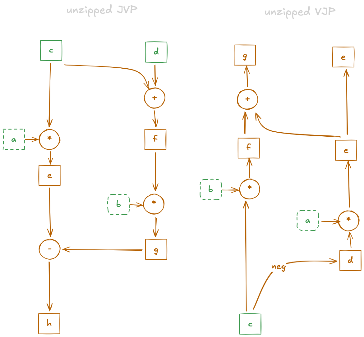
The article you've been reading provides clear code examples for implementing custom VJPs for the core components of a simple neural network.
Everything You Need to Know About Backpropagation | George Assaad
This part of the article translates the theory directly into JAX code.
Please study the section "Implementing Custom VJPs in JAX" and the two subsequent sections, "Deriving the Softmax Cross-Entropy Gradient" and the code block that follows it. Pay special attention to: The Linear implementation: see how Linear_fwd saves W and x as residuals, and how Linear_bwd uses them to compute the gradients grad_W and grad_x. The Tanh implementation: notice how the output of the forward pass a is itself the residual needed for the backward pass. The softmax_cross_entropy implementation: this is a prime example of combining operations for numerical stability. The final gradient p - y is remarkably simple and much more stable to compute than differentiating through a separate softmax and log. Notice how the backward rule for the label input is None, as it's not a parameter we need to differentiate with respect to.
4. A Complete Example
With these custom-defined primitives, you can build and train a full neural network. JAX's grad function will seamlessly use your custom VJP rules wherever it encounters the decorated functions, composing them correctly with its own default rules for other operations (like jnp.mean).
The article concludes with a complete, working script that trains a two-layer network on MNIST using only the Linear, Tanh, and softmax_cross_entropy functions we just defined.
Everything You Need to Know About Backpropagation | George Assaad
This final code block demonstrates the practical application of custom VJPs in a full training loop.
Please review the code in the final section, "Putting It All Together: A Full Example". You don't need to run it, but observe how the update_step function, which uses value_and_grad, works perfectly with our forward_pass and batch_loss_fn that are built entirely from custom VJP functions. This shows the power and elegance of JAX's compositional design.
This ability to drop in custom rules without disrupting the rest of the ecosystem is a hallmark of well-designed functional frameworks and a cornerstone of JAX's flexibility.
Conclusion
In this lesson, you've unlocked one of the most powerful features of JAX's automatic differentiation system. By moving beyond the high-level grad API, you've gained the ability to precisely control the backpropagation process.
Key Takeaways:
- Backpropagation is an efficient implementation of reverse-mode AD, which works by chaining together Vector-Jacobian Products (VJPs).
- Efficient VJP implementations rarely materialize the full Jacobian matrix. Instead, they use analytical shortcuts to compute the effect of multiplying by the Jacobian transpose.
- JAX's
@jax.custom_vjpdecorator allows you to define your own backward pass for a function. - This involves defining a
fwdrule to compute the output and save necessaryresiduals, and abwdrule to compute input gradients using theresidualsand the upstream gradientg. - This technique is invaluable for performance optimization (e.g.,
Linear), numerical stability (e.g.,softmax_cross_entropy), and implementing novel algorithms.
In our next lesson, we will look at a related, but much simpler, concept: how to prevent gradients from flowing through certain parts of your model altogether using jax.lax.stop_gradient. This is a common requirement in techniques like self-supervised learning or when freezing parts of a model during fine-tuning.