Automatic Differentiation with JAX: Jacobians and Hessians

1. Computing Full Jacobians

In the last lesson, we saw that jvp computes a Jacobian-vector product, $J_f(x)v$, and vjp computes a vector-Jacobian product, $v^T{J}_f(x)$. A natural question arises: how do we obtain the full Jacobian matrix $J_f(x)$ itself?

The direct approach would be to probe the matrix column by column or row by row.

• To get the $i$-th column, we can compute $J_f(x)e_i$, where $e_i$ is the $i$-th standard basis vector (a one-hot vector). This requires one jvp call per input dimension.
• To get the $j$-th row, we can compute $e_j^T{J}_f(x)$, where $e_j$ is the $j$-th standard basis vector. This requires one vjp call per output dimension.

While this works, it's cumbersome and inefficient to implement with a Python loop. JAX provides a much more elegant and efficient solution by composing these operations with jax.vmap. This leads to two distinct functions for computing the Jacobian.

jax.jacfwd: Forward-Mode Jacobian

jax.jacfwd computes the Jacobian using forward-mode AD. Conceptually, it vectorizes the jvp function over a set of standard basis vectors for the input. This is equivalent to building the Jacobian column by column, but all in one highly optimized pass.

Because it's built on jvp, its performance characteristics are the same: it is efficient for functions with "tall" Jacobians, where the number of outputs is significantly larger than the number of inputs ($m>n$).

jax.jacrev: Reverse-Mode Jacobian

Conversely, jax.jacrev computes the Jacobian using reverse-mode AD. It vectorizes the vjp's pullback function over a set of standard basis vectors for the output. This is equivalent to building the Jacobian row by row in a single pass.

Since jacrev is built on vjp, it is efficient for functions with "wide" Jacobians, where the number of inputs is much larger than the number of outputs ($n>m$). This is the common case in machine learning, where a model with millions of parameters ($n$) is optimized against a single scalar loss ($m=1$). In this scenario, jax.grad(f) is equivalent to jax.jacrev(f) (with some trivial reshaping).

The JAX documentation provides a concise guide to using these functions.

For functions with roughly square Jacobians ($n\approx m$), jacfwd often has a slight performance advantage due to its lower memory overhead. The following benchmark plots clearly illustrate this trade-off in practice.

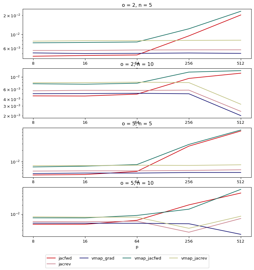
Let's analyze these plots based on what we've learned. Assume a function $f:{\mathbb{R}}^{n\cdot p}\to {\mathbb{R}}^{o\cdot p}$.

1. Top two plots (o=2, n=5 and o=2, n=10): Here, the input dimension (n*p) is larger than the output dimension (o*p), creating a "wide" Jacobian. As predicted, jacrev (pink) is significantly faster than jacfwd (red).
2. Third plot (o=5, n=5): Here we have a "square" Jacobian. The performance of jacfwd and jacrev is very close, with jacfwd showing a slight edge.
3. Bottom plot (o=5, n=10): A "wide" Jacobian again. jacrev is the clear winner.

These empirical results perfectly validate the theoretical performance models of forward- vs. reverse-mode AD.

2. Computing Hessians

The Hessian matrix is the second derivative of a scalar-valued function $f:{\mathbb{R}}^n\to \mathbb{R}$. Mathematically, it is the Jacobian of the gradient:

Since the gradient function $\nabla f$ is a mapping from ${\mathbb{R}}^n\to {\mathbb{R}}^n$, its Jacobian (the Hessian) will be an $n\times n$ matrix.

Given this relationship, we can compute a Hessian by composing our Jacobian functions. This gives us a few options: jacfwd(jacfwd(f)), jacrev(jacrev(f)), jacfwd(jacrev(f)), and jacrev(jacfwd(f)). Is there an optimal choice?

Let's analyze the most common and efficient composition: jacfwd(jacrev(f)).

1. Inner function: g = jacrev(f). For a function $f:{\mathbb{R}}^n\to \mathbb{R}$, we are computing the Jacobian of a function with a very "wide" 1 x n shape. As we know, jacrev is the most efficient choice for this. The result is the gradient function, $g=\nabla f$, which maps ${\mathbb{R}}^n\to {\mathbb{R}}^n$.
2. Outer function: jacfwd(g). We are now computing the Jacobian of the gradient function $g$, which has a "square" n x n Jacobian. For square Jacobians, jacfwd is generally the most efficient choice.

This "forward-over-reverse" strategy is typically the most performant way to compute a dense Hessian. JAX conveniently wraps this logic in a single function, jax.hessian.

The following tutorial provides a practical demonstration of using these functions.

The "Autodiff Cookbook" also formalizes this concept.

3. A Look Under the Hood

A key aspect of JAX's design, which should appeal to your interest in system internals, is that these powerful transformations are themselves composed of simpler ones. jacfwd and jacrev are not monolithic functions; they are elegantly implemented using jvp, vjp, and vmap.

• jacfwd is implemented by applying vmap to jvp. It maps the jvp operation across a batch of standard basis vectors fed into the tangents argument.
• jacrev is implemented by applying vmap to the pullback function returned by vjp. It maps the pullback over a batch of standard basis vectors fed into the cotangents.

This compositional approach is a hallmark of JAX's design philosophy. Understanding it reveals that JAX isn't "magic"; it's a small, consistent set of orthogonal primitives (jit, grad, vmap, pmap) that can be combined to express a vast range of complex computations.

Conclusion

In this lesson, we bridged the gap between the low-level jvp and vjp primitives and the high-level task of computing full derivative matrices. You are now equipped to compute Jacobians and Hessians of any JAX function and, more importantly, to reason about the most efficient way to do so.

Key Takeaways:

• jax.jacfwd (forward-mode) and jax.jacrev (reverse-mode) compute full Jacobian matrices. The choice between them is a performance optimization based on the Jacobian's shape: jacfwd for tall matrices ($m>n$) and jacrev for wide matrices ($n>m$).
• jax.hessian computes the Hessian of a scalar-valued function. It is a convenience wrapper that efficiently composes jacfwd(jacrev(f)), leveraging the strengths of both autodiff modes.
• These high-level transformations are not black boxes; they are themselves compositions of JAX's fundamental primitives (jvp, vjp, and vmap), showcasing the power and elegance of JAX's functional design.

While we can now compute a full, dense Hessian matrix, for the very large-scale models common in deep learning (with millions or billions of parameters), materializing an $n\times n$ Hessian is often computationally infeasible. Many advanced optimization algorithms, however, don't require the full Hessian, but rather its product with a vector. In the next lesson, you will learn how to compute these Hessian-vector products efficiently, a critical technique for second-order optimization at scale.