Welcome to our new module, where we will explore the engine that powers modern machine learning: automatic differentiation. In the previous module, we established a solid foundation in JAX's data structures, culminating in debugging the common errors that arise when manipulating pytrees. Now, we shift our focus from the data to the computation—specifically, how JAX computes gradients with remarkable efficiency and flexibility.
This first lesson addresses the heart of automatic differentiation. We will distinguish between its two fundamental modes, forward-mode and reverse-mode, and understand their JAX counterparts: jvp and vjp. You already know that jax.grad is the go-to for training models, but by the end of this lesson, you will understand why it works the way it does and why it is a special case of the more general reverse-mode. Most importantly, you will learn to reason about the computational complexity of each mode, enabling you to choose the correct tool for any given differentiation task based on the shape of the problem.
1. The World of Differentiation
Before diving into the mechanics, it's useful to contextualize automatic differentiation (AD). As you know from your mathematical and practical experience, we need derivatives for optimization. While manual derivation is feasible for simple models, it's intractable for deep neural networks. Other automated methods have significant drawbacks.
The following video provides an excellent, concise overview of the landscape, contrasting automatic differentiation with its main alternatives: numerical and symbolic differentiation.
What is Automatic Differentiation?
This video from the channel Ari Seff succinctly explains why automatic differentiation is the preferred method for machine learning.
Please watch the first part of the video, from the beginning until the introduction of forward and reverse modes at this timestamp. As you watch, focus on the critiques of: Numerical Differentiation: Issues with truncation and rounding errors, but more critically, the O(n) computational cost for a function with n inputs. Symbolic Differentiation: The problem of "expression swell," where the symbolic representation of the derivative can become exponentially larger than the original function.
Automatic differentiation elegantly avoids these pitfalls. It computes derivatives to machine precision, like symbolic methods, but with a computational cost that is only a small constant factor more than evaluating the function itself. It achieves this by systematically applying the chain rule to the sequence of primitive operations that constitute your program. The key to understanding AD lies in visualizing this sequence as a computational graph.
2. The Computational Graph
A computational graph is a directed acyclic graph (DAG) where nodes represent primitive operations (e.g., +, *, log, sin) or input variables, and edges represent the flow of data between them. Evaluating the function corresponds to a forward pass through this graph, from inputs to outputs.
This representation is fundamental because it makes the dependencies between all variables explicit, providing the structure needed to apply the chain rule. The following lecture explains this concept clearly.
Lecture 4 - Automatic Differentiation
This segment from the Deep Learning Systems Course at UW introduces the computational graph, the foundational structure for automatic differentiation.
Watch the segment from this timestamp that defines and demonstrates the evaluation of a computational graph. The example traces the flow of values through the nodes, which is precisely the "forward pass" of a computation.
With the computational graph as our framework, we can now explore the two primary ways to traverse it to compute derivatives.
3. Forward-Mode AD: Jacobian-Vector Products (JVP)
Forward-mode automatic differentiation is conceptually the more direct approach. It traverses the computational graph from inputs to outputs, just like a standard function evaluation. However, at each node, it computes not only the primal value (the value of the intermediate variable) but also its derivative, or "tangent," with respect to a single input variable.
Let's consider a function . A single pass of forward-mode AD computes the derivatives of all outputs with respect to one input.
Lecture 4 - Automatic Differentiation
The same lecture provides an excellent step-by-step trace of the forward-mode algorithm on the example computational graph.
Watch the portion explaining forward-mode AD from this timestamp. Notice how a new quantity, v_dot (representing \partial v / \partial x_1), is computed alongside each primal value v. The rule at each node is a direct application of the chain rule based on the derivatives of its inputs.
This process is more formally known as computing a Jacobian-vector product (JVP). The Jacobian matrix of a function at a point is the matrix of all first-order partial derivatives. The JVP is the result of multiplying this Jacobian by a "tangent" vector .
A forward-mode AD pass with the input tangent vector set to a one-hot vector (i.e., [0, ..., 1, ..., 0]) effectively computes , which is precisely the i-th column of the Jacobian.
This means that to compute the full Jacobian, we would need passes of forward-mode AD, one for each input dimension. This makes it efficient when the number of inputs is small.
In JAX, the primitive for this is jax.jvp.
The Autodiff Cookbook — JAX documentation
The JAX documentation gives a clear mathematical and code-based explanation of JVPs.
Please read the section on JVPs in math and code. Pay close attention to the Haskell-like type signature: jvp :: (a -> b) -> a -> T a -> (b, T b). This elegantly captures the operation: jvp takes a function, a primal input a, and a tangent input T a, and returns a pair of the primal output b and the tangent output T b. Also, note the discussion on computational complexity: the cost is about 3x the original function evaluation and has a low memory footprint.
The key takeaway for forward-mode is its efficiency for functions with "tall" Jacobians, where the input dimension n is much smaller than the output dimension m.
4. Reverse-Mode AD: Vector-Jacobian Products (VJP)
Reverse-mode AD is the workhorse of deep learning and what you implicitly use when calling .backward() in PyTorch or jax.grad in JAX. It's more complex, involving two stages.
- Forward Pass: The function is evaluated as usual, from inputs to outputs. However, the values of all intermediate variables (the primals) and the structure of the computational graph are stored in memory.
- Backward Pass: The chain rule is applied in reverse, propagating derivatives from the final output back to the inputs. The derivative of the final output with respect to an intermediate variable is called its "adjoint" or "cotangent."
A single reverse-mode pass (one forward + one backward) computes the derivative of one scalar output with respect to all input variables.
Lecture 4 - Automatic Differentiation
This is the most critical part of the lecture, as it details the mechanism of reverse-mode AD.
Please watch the two sections explaining reverse-mode AD, starting from this timestamp. The first part walks through the backward pass, introducing the v_bar notation for adjoints. Notice how it starts from the output (where the adjoint is 1) and works backward. The second part provides the formal derivation for fan-out nodes (where one variable is used in multiple subsequent operations). This confirms mathematically why the incoming gradients must be summed.
This process is formally known as a Vector-Jacobian product (VJP). It computes the product of a "cotangent" vector with the Jacobian matrix.
A reverse-mode AD pass with the output cotangent vector set to 1.0 (for a scalar output) computes , which is the gradient , a single row of the Jacobian.
This makes reverse-mode incredibly efficient for functions with few outputs and many inputs, which is exactly the case when training a neural network: you have millions of parameters (inputs, n is large) and a single scalar loss (output, m=1).
In JAX, the primitive for this is jax.vjp.
The Autodiff Cookbook — JAX documentation
This section of the documentation contrasts VJPs with JVPs and explains the JAX primitive.
Read the section on VJPs in math and code. Again, the type signature is revealing: vjp :: (a -> b) -> a -> (b, CT b -> CT a). vjp takes a function and a primal input a, and returns the primal output b along with a function (the "pullback" function) that can map an output cotangent CT b to an input cotangent CT a. This functional nature is a core tenet of JAX. Note the mention of the memory cost, which scales with the depth of the computation.
jax.grad is simply a convenience wrapper around jax.vjp for the common case of scalar-valued functions, where the output cotangent is implicitly 1.0.
5. Choosing the Right Mode: A Summary
The choice between forward- and reverse-mode is a direct trade-off based on the shape of your function's Jacobian.
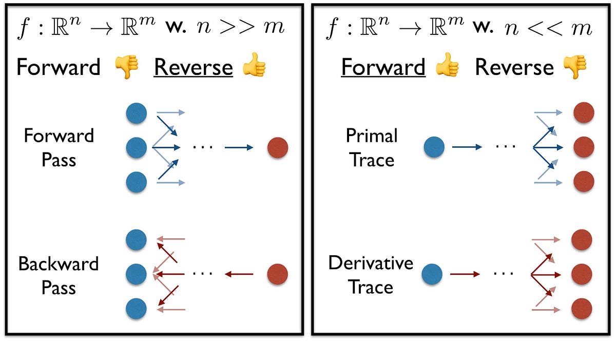
Here is a summary of the key distinctions:
| Feature | Forward-Mode (JVP) | Reverse-Mode (VJP) |
|---|---|---|
| JAX Primitive | jax.jvp |
jax.vjp (jax.grad is a wrapper) |
| Direction | Propagates derivatives from inputs to outputs. | Propagates derivatives from outputs to inputs. |
| Computes per Pass | One column of the Jacobian (). | One row of the Jacobian (). |
| Efficient for | "Tall" Jacobians: n << m (many outputs, few inputs). |
"Wide" Jacobians: n >> m (many inputs, few outputs). |
| Memory Cost | Low. Independent of computation depth. | High. Proportional to computation depth (must store primals). |
| ML Use Case | Computing Hessian-vector products. | Standard gradient-based optimization of scalar loss functions. |
Conclusion
In this lesson, we have dissected the two fundamental modes of automatic differentiation. You now understand the core mechanics of both forward-mode (JVP) and reverse-mode (VJP), how they relate to the computational graph, and their distinct performance characteristics.
Key Takeaways:
- Automatic differentiation operates on a computational graph, applying the chain rule systematically.
- Forward-mode (JVP) computes one column of the Jacobian per pass. It is efficient for functions with "tall" Jacobians (
n << m). - Reverse-mode (VJP) computes one row of the Jacobian per pass. It is efficient for functions with "wide" Jacobians (
n >> m), making it the standard for training deep learning models.jax.gradis a specialized VJP. - The choice between modes is a computational trade-off determined by the relative sizes of the function's input (
n) and output (m) dimensions.
With this foundational understanding of jvp and vjp, we are now ready to build higher-level differentiation tools. In the next lesson, we will see how JAX cleverly composes these two primitives to efficiently compute full Jacobian and Hessian matrices, giving you complete control over the differentiation process.