Handling Corporate Actions in Historical Data

The Problem with Raw Price Data

Imagine your strategy sees a stock price drop 75% in a single day. It would almost certainly trigger a sell signal. But what if that "drop" was actually a 4-for-1 stock split? The company's value didn't change, and as a shareholder, your total investment value remained the same; you just own four times as many shares at a quarter of the price. The raw price chart, however, tells a dangerously misleading story.

Corporate actions are events initiated by a company that affect its securities. For our purposes, the two most important are:

1. Stock Splits: The company changes the number of shares outstanding, which proportionally changes the price per share.
2. Dividends: The company distributes a portion of its profits to shareholders in cash.

Both events change the stock's price on the chart without reflecting a true change in the company's underlying value or an investor's total wealth. Let's see how to correct for each.

Adjusting for Stock Splits

A stock split changes the number of a company's shares without changing its market capitalization. For instance, in a 2-for-1 split, every shareholder gets an additional share for each one they own, and the stock price is halved. The total value of their holding is unchanged.

To create a continuous price series, we must adjust all historical prices prior to the split to be comparable to the post-split prices. The QuantStart article "Understanding Equities Data" provides a clear explanation of this.

As the article explains, the adjustment is straightforward. For a 2-for-1 split, the factor is $\frac{1}{2}=0.5$. You multiply all historical open, high, low, and close prices before the split date by 0.5. For a 4-for-1 reverse split like the one in the VXX chart, it's an M-for-N split (1-for-4), so the factor is $\frac{4}{1}=4$. You would multiply all prior historical prices by 4 to bring them in line with the new, higher price level.

Adjusting for Dividends

Dividends are more subtle but just as important. When a company pays a dividend, it is transferring cash from its accounts to its shareholders. This means the company is now worth less by the total amount of the dividend paid. On the ex-dividend date (the first day the stock trades without the right to receive the upcoming dividend), the stock price will typically drop by approximately the dividend amount.

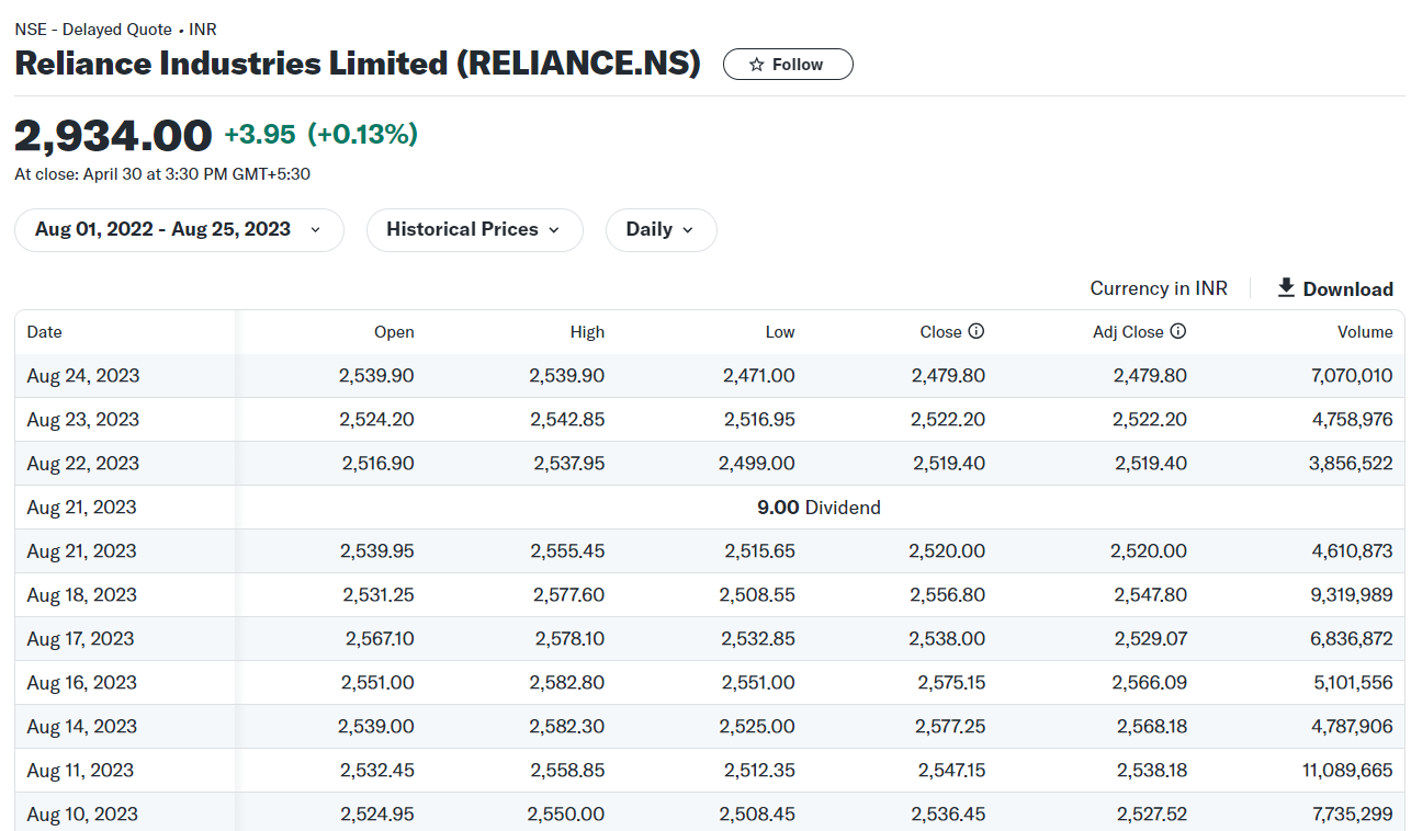
A naive backtest would see this price drop as a capital loss. However, the shareholder's total wealth didn't change—the loss in stock value was offset by the cash received. To correctly model historical returns, we must adjust for this.

A simple subtraction of the dividend from all prior prices is incorrect and can lead to nonsensical results like negative prices over long periods. The correct method, used by professional data providers, involves applying a multiplicative factor. The blog post "Analyzing intraday and overnight stock returns with pandas" provides an excellent, code-centric walkthrough of this exact process.

The key takeaway is that both splits and dividends are handled by applying a cumulative product of adjustment factors backwards in time. This ensures that the adjusted price series represents the total return of the investment, which is the only valid basis for testing a trading strategy.

The Practical Solution: Let Your Data Provider Do the Work

Understanding the theory is vital for diagnosing data issues. However, when building your system, you rarely need to perform these calculations yourself. Your proficiency in Python can be leveraged by using libraries that handle this automatically.

Most reputable financial data providers offer both raw prices and adjusted prices. The yfinance library for Python makes accessing this incredibly simple.

The following short clip from QuantInsti demonstrates the easiest way to get fully adjusted data.

When you use auto_adjust=True, yfinance returns a DataFrame with the OHLCV data already adjusted using the standardized methods we've just discussed. It also removes the Dividends and Stock Splits columns, as their effects are already baked into the prices.

For backtesting the logic of a strategy, you should always use this fully adjusted price series.

Conclusion

In this lesson, we completed the final, critical step of data preparation: adjusting for corporate actions. An unadjusted price series is deceptive and will doom any backtest to failure.

Here are the key takeaways:

• Corporate actions like stock splits and dividends create artificial price jumps in raw historical data.
• Stock splits are corrected by multiplying all prior prices by a ratio factor (e.g., 0.5 for a 2-for-1 split).
• Dividends are corrected by applying a cumulative multiplicative factor, calculated as $1-(\text{dividend}/\text{price})$, backwards in time.
• The goal of adjustment is to create a continuous total return series, which is the only valid foundation for backtesting strategy performance.
• In practice, you can use a library like yfinance with the auto_adjust=True setting to automatically receive a fully adjusted and clean dataset.

We now have a pristine, research-ready price series. It is clean, time-aligned, and correctly adjusted. With this solid foundation, we can finally begin calculating meaningful metrics. In our next lesson, we will use this data to measure one of the most fundamental concepts in finance: historical and rolling volatility.