Measuring Volatility

What is Volatility?

In simple terms, volatility measures how much an asset's price swings around its average. A highly volatile stock sees large, rapid price changes, while a low-volatility stock tends to be much more stable. For a trader, volatility is synonymous with both risk and opportunity.

Finance professionals distinguish between two main types of volatility:

1. Historical Volatility: This is a backward-looking measure calculated from past price data. It tells us how volatile an asset has been.
2. Implied Volatility: This is a forward-looking measure derived from options prices. It represents the market's consensus on how volatile an asset is expected to be in the future.

In this lesson, we will focus exclusively on historical volatility, as it's a critical component for backtesting and risk management that can be calculated directly from the price data we've already prepared.

To get a formal handle on the concept, please begin by reading the introductory sections of the SimTrade blog post on Historical Volatility.

The Calculation: From Returns to Volatility

As the article highlights, volatility is not calculated on prices, but on returns. Specifically, it is the standard deviation of the logarithmic returns over a certain period. The process involves three main steps:

1. Calculate Logarithmic Returns: For each period (e.g., daily), calculate the log return: $r_t=\ln (\frac{P_t}{P_{t-1}})$.
2. Calculate Standard Deviation: Compute the standard deviation of these returns over a chosen lookback window.
3. Annualize the Volatility: Scale the result to an annual figure for comparability.

The standard deviation gives us the volatility for the period of the returns (e.g., daily volatility from daily returns). To make it meaningful and comparable across different assets and timeframes, we annualize it. This is done by multiplying the daily volatility by the square root of the number of trading days in a year, which is conventionally taken as 252.

The SimTrade article provides a clear walkthrough of this.

From Theory to Practice: Rolling Volatility in Python

Calculating a single volatility number over your entire dataset (unconditional volatility) gives you a long-term average, but it's not very useful for active trading. Volatility is not static; it changes over time, with quiet periods followed by turbulent ones. To capture this dynamic nature, we use a rolling volatility.

A rolling volatility is calculated using a moving window. For example, a 21-day rolling volatility would, for each day, calculate the standard deviation of the log returns of the preceding 21 trading days. This gives us a time series of volatility, allowing us to see how risk is evolving.

Given your proficiency in Python, you'll find the pandas library makes this calculation incredibly straightforward. The following video by Matt Macarty provides a concise demonstration of the .rolling() method, which is the core of this technique.

Combining what you've learned, the complete process in pandas is:

1. Calculate log returns: log_returns = np.log(df['Adjusted Close'] / df['Adjusted Close'].shift(1))
2. Calculate rolling annualized volatility: rolling_vol = log_returns.rolling(window=21).std() * np.sqrt(252)

The image below shows both the Python code for this calculation and the resulting plot. This is exactly the kind of output you can now generate to visualize how an asset's risk profile has changed over time.

An Improvement: Exponentially Weighted Moving Average (EWMA)

The simple rolling window (a Simple Moving Average, or SMA) has one notable drawback: a single large return shock will stay in the calculation for the entire window length and then abruptly disappear, causing a sudden drop in the volatility reading even if nothing happened in the market on that day. This is sometimes called a "ghosting" or "leverage" effect.

A more responsive and widely-used method is the Exponentially Weighted Moving Average (EWMA). EWMA calculates the standard deviation by giving more weight to recent returns and exponentially less weight to older ones. This means shocks fade out smoothly, and the volatility estimate adapts more quickly to new market information.

The EODHD article "Estimate Volatility with SMA and EWMA in Python" provides an excellent comparison of these two approaches.

For most quantitative trading applications, EWMA-based volatility is preferred over the simple rolling window due to its responsiveness and smoother decay.

Why This Matters for Your Trading System

Measuring volatility isn't just an academic exercise. It's a practical tool that directly informs trading decisions. By quantifying the market's current risk level, you can:

• Adjust Position Size: Take smaller positions in highly volatile markets and larger positions in calmer ones. This is known as "volatility targeting" and is a powerful risk management technique we will cover later.
• Filter Trading Signals: Some strategies work best in low-volatility, mean-reverting environments, while others (like breakouts) thrive on high volatility. You can use a volatility measure as a filter to turn your strategy on or off.
• Set Dynamic Exits: Stop-loss and take-profit levels can be set as a multiple of the current volatility (e.g., place a stop at 2x the daily volatility), making them adapt to changing market conditions.

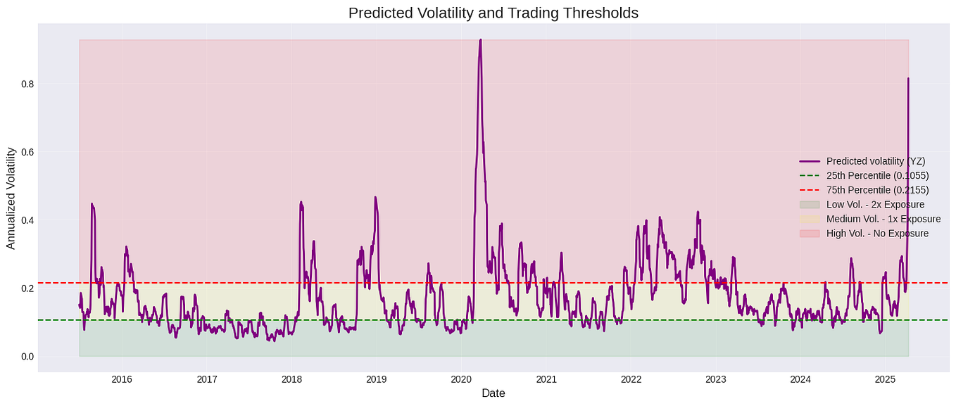
The plot below shows a practical application of this idea, where predicted volatility is used to define different trading regimes, each with a different level of capital exposure.

Conclusion

In this lesson, you have learned how to measure and interpret one of the most critical metrics in finance.

Here are the key takeaways:

• Volatility is the standard deviation of an asset's logarithmic returns and is the primary measure of its price risk.
• Volatility is annualized by multiplying the daily volatility by the square root of 252, allowing for standardized comparisons.
• Rolling volatility provides a dynamic view of how an asset's risk evolves over time, which is far more useful for trading than a single static value.
• EWMA-based volatility is generally superior to a simple rolling window because it adapts more quickly to new information and avoids the abrupt "ghosting" effect of old data points dropping out of the window.
• Measuring volatility is a cornerstone of risk management, influencing position sizing, strategy filtering, and exit placement.

You have moved from simply processing data to extracting a meaningful risk metric from it. In our next lesson, we will explore another crucial aspect of risk: drawdown. While volatility measures the general magnitude of price swings, drawdown measures the specific pain of a losing streak from a portfolio's peak to its trough.