In our last lesson, we established the importance of logarithmic returns and learned how to calculate them from a price series. This was our first step in transforming raw price data into a usable input for quantitative models. However, the reliability of those returns—and any analysis built upon them—depends entirely on the quality of the underlying price data.
This lesson addresses a critical, non-negotiable step in building any trading system: ensuring data integrity. Real-world financial data is often messy. It can have gaps, errors, and inconsistencies that can silently corrupt your backtest results and lead to flawed conclusions. We will focus on performing data integrity checks and, most importantly for your intraday trading goals, mastering time alignment for historical price feeds. By the end of this lesson, you will have a robust process for cleaning and preparing time-series data for analysis.
"Garbage In, Garbage Out": The Problem of Dirty Data
The adage "garbage in, garbage out" is paramount in quantitative finance. Before you can derive any insights, you must first become a data janitor. Historical price data, especially at intraday frequencies, can suffer from several common issues:
- Missing Values (
NaN): A specific data point within a bar might be missing. For example, a 1-minute OHLC bar could be missing itslowprice. - Missing Timestamps: Entire time intervals can be absent from the dataset. For an intraday trader, a missing 1-minute bar at a critical time like the market open can completely invalidate a strategy's backtest.
- Timezone Ambiguity: Timestamps might be recorded in UTC, the local exchange time (e.g., America/New_York), or without any timezone information at all (naive). Misinterpreting timezones can lead to you analyzing data from the wrong hours.
- Irregular Intervals: Data that is supposedly "1-minute" may have timestamps that are slightly off, such as
09:30:01,09:31:00,09:31:59.
Let's look at an example of what real 1-minute historical data can look like.
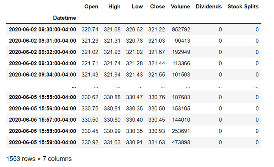
Our goal is to create a clean, continuous, and uniformly-spaced time series that accurately reflects the trading periods we care about. We will tackle this using the powerful time-series tools in the Pandas library.
Handling Missing Data (NaN)
The first and most straightforward problem is when a value is explicitly missing and represented in a Pandas DataFrame as NaN (Not a Number). We have several strategies to handle this, ranging from simple to more sophisticated.
The following video from the codebasics channel provides an excellent overview of the primary methods in Pandas for handling missing data.
Python Pandas Tutorial 5: Handle Missing Data: fillna, dropna, interpolate
This tutorial, "Handle Missing Data: fillna, dropna, interpolate," offers clear, practical examples of the most common techniques.
Please watch the following segments: Filling NaNs: Watch from the introduction to fillna through the explanation of forward-fill (ffill) and backward-fill (bfill). Forward-filling is particularly common for price data, as it assumes the price remained at its last known value, which is often a reasonable starting assumption. Interpolation: Continue watching from the interpolate method. Pay close attention to the difference between standard linear interpolation and method='time'. Time-based interpolation is generally superior for financial time series as it correctly weights the values based on the duration of the time gap.
As the video demonstrates, blindly dropping rows with dropna() is usually a poor choice, as you might discard a mostly valid data point. fillna(method='ffill') and interpolate(method='time') are your go-to tools for intelligently filling in missing values within your dataset.
Aligning the Time Index: Handling Missing Bars
A more complex and common issue in intraday data is the complete absence of a timestamp. Your data might jump from 09:35:00 to 09:37:00, entirely skipping the 09:36:00 bar. To fix this, we need to conform our data to a perfect, complete time index.
The process involves two main steps:
- Creating a complete, regular date range that represents every timestamp we expect to see.
- Using this new index to
reindexour original DataFrame. This will insert rows for the missing timestamps, withNaNvalues in all the data columns.
Once we've done this, the problem of missing rows is transformed into the problem of missing values, which we already know how to solve with fillna or interpolate.
The codebasics video you just watched also covers this exact technique.
Python Pandas Tutorial 5: Handle Missing Data: fillna, dropna, interpolate
Let's revisit the video to see how to create and use a complete time index.
Watch the final section on inserting missing dates. The example uses daily data, but the principle is identical for intraday minute-by-minute data. The key functions are pd.date_range() to create the ideal index and df.reindex() to apply it.
This reindex and fillna combination is a fundamental pattern for cleaning financial time series data.
Mastering Intraday Resampling and Alignment
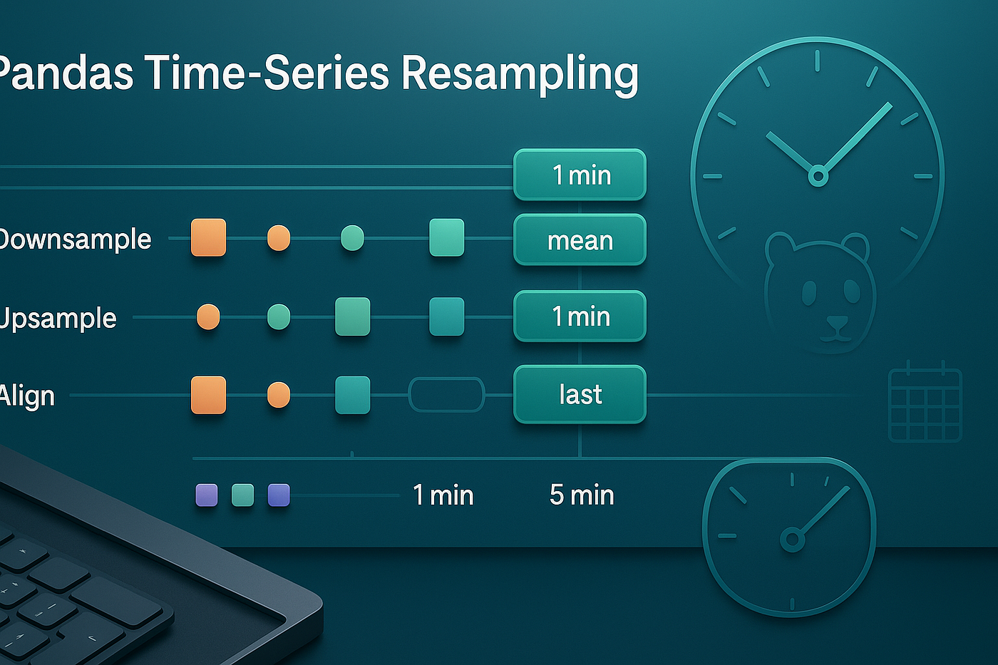
For your goal of intraday trading, simply filling gaps isn't enough. You need to be precise about how you define your time bars (or "candles"). This is where resampling comes in. Resampling is the process of changing the frequency of your time series data.
Corey Schafer's tutorial provides a very clear introduction to the resample() method and how to apply aggregation functions.
Python Pandas Tutorial (Part 10): Working with Dates and Time Series Data
This video, "Working with Dates and Time Series Data," clearly explains the concept of resampling and aggregation.
Watch the segment from resampling. This will show you how to change the data's frequency (e.g., from hourly to daily or weekly) and apply different aggregation functions (mean, max, sum, etc.) to different columns.
Building on that foundation, let's dive into the specifics required for generating clean OHLCV (Open, High, Low, Close, Volume) bars, which is a classic downsampling task.
The following article offers a set of practical, "battle-tested" recipes for cleaning time-series data in Pandas. We'll focus on the recipes most relevant to financial data.
8 Pandas Time-Series Recipes for Clean Resampling
This article provides robust, code-centric solutions for common time-series data cleaning tasks.
Please read the following sections: "The honest downsample": Read this section to see how to properly aggregate high-frequency data into OHLC-style bars using .resample(...).agg({...}). This is how you would convert tick data or 1-minute data into 5-minute or 15-minute bars. Labeling and Alignment: Read section 3. The label, closed, and origin parameters are absolutely critical for financial data. They control whether the timestamp represents the start or end of the bar and ensure that your 5-minute bars align consistently across different days (e.g., always at :00, :05, :10...). Business Time: Read section 5. This demonstrates two essential functions for intraday strategies: df.between_time("09:30", "16:00"): This allows you to easily filter your data to include only the official trading hours. resample("B"): The "B" frequency code stands for "business day," which automatically skips weekends. Timezone Safety: Read section 6. The rule here is non-negotiable: Always make your timestamps timezone-aware before you resample. You should localize your data to the correct exchange timezone (e.g., 'America/New_York' for US stocks) to avoid errors caused by Daylight Saving Time transitions.
A Practical Workflow for Intraday Data Cleaning
Let's combine everything we've learned into a step-by-step checklist you can implement in Python for cleaning an intraday price feed.
- Load Data: Load your CSV or data source into a Pandas DataFrame.
- Parse and Index:
- Convert your timestamp column to datetime objects using
pd.to_datetime(df['time_column'], format=...). Providing theformatstring is crucial for non-standard timestamp formats. - Set this column as the DataFrame index:
df.set_index('time_column', inplace=True).
- Convert your timestamp column to datetime objects using
- Handle Timezones:
- If your data is timezone-naive but in UTC, localize it:
df.tz_localize('UTC'). - Convert it to the exchange's local time:
df = df.tz_convert('America/New_York'). This is the correct index for analysis.
- If your data is timezone-naive but in UTC, localize it:
- Filter Trading Hours:
- Isolate the regular trading session:
df = df.between_time('09:30', '16:00').
- Isolate the regular trading session:
- Create a Full, Clean Index:
- Group data by date and, for each day, create a complete 1-minute index from market open to close.
- Reindex each day's data to this complete index. This will introduce
NaNs for missing bars.
- Fill Gaps:
- Apply
ffill()to the price columns (Open,High,Low,Close) to carry the last known price forward. - Apply
fillna(0)to theVolumecolumn, as missing bars likely had zero trading volume.
- Apply
- Verify:
- Run
df.isnull().sum()to confirm there are no more missing values in your cleaned DataFrame.
- Run
By following this process, you transform a potentially messy and unreliable raw data feed into a high-quality, research-ready dataset.
Conclusion
In this lesson, we moved from calculating returns to ensuring the data we use for those calculations is sound. You've learned that data integrity is not an optional step but a foundational requirement for any quantitative trading strategy.
Here are the key takeaways:
- Real-world financial data is imperfect and requires cleaning.
- Missing values (
NaN) can be handled withfillna(especially forward-fill) or more advancedinterpolatemethods. - Missing timestamps are fixed by creating a complete time index and using
reindex, which turns the problem back into one of handlingNaNs. - For intraday data, you must handle timezones correctly (
tz_convert) and filter for trading hours (between_time) before resampling. - The
resamplemethod, combined with.agg(), is your primary tool for creating clean OHLCV bars at any desired frequency.
Our data is now clean and correctly aligned in time. However, there is one final adjustment we must make to our historical prices before they are ready for backtesting: accounting for corporate actions. In our next lesson, we will learn how to adjust historical prices for stock splits and dividends to create a continuous and accurate price history.