Calculating Logarithmic Returns

Welcome to your first lesson. This course is designed to equip you with the practical skills needed to build and evaluate your own algorithmic trading systems. We will start from the ground up, ensuring each concept is not only understood theoretically but is also something you can immediately implement in Python.

This first module focuses on the essential building blocks of quantitative analysis: performance metrics and data handling. Today, we'll tackle the most fundamental of these: calculating asset returns. You'll learn why logarithmic returns are the standard in quantitative finance, how they differ from simple returns, and how to compute them. This concept is the starting point for almost every subsequent topic in this course, from measuring volatility to backtesting strategies.

Simple Returns vs. Logarithmic Returns

Before diving into logarithmic returns, let's start with the more intuitive concept: the simple return. This is the straightforward percentage gain or loss of an asset over one period.

The formula is:

R_{simple} = \frac{P _{t}}{P _{t - 1}} - 1

where $P_{t}$ is the price at the current time $t$ , and $P_{t - 1}$ is the price at the previous time $t - 1$ .

Simple returns are easy to understand, but they have a significant drawback for financial analysis: they are not time-additive. For example, if a stock gains 10% on day one and loses 10% on day two, the total return is not 0%. Instead, you must compound the returns: $(1 + 0.10) \times (1 - 0.10) - 1 = - 0.01$ , or a 1% loss. This multiplicative nature makes analyzing returns over many periods cumbersome.

To address this, quantitative analysts use logarithmic returns (or log returns).

A brief overview on simple returns and log ...

This article from Medium provides a concise definition of both simple and log returns.

Please read the first two sections, Simple Return and Log Return, to familiarize yourself with their definitions and formulas.

As you've just read, the log return is calculated as the natural logarithm of the price ratio. This simple transformation gives it some very powerful properties.

The Intuition: From Compounding to Continuous Returns

So, why the natural logarithm? The answer lies in the concept of continuous compounding. Stock prices don't just change once per day; they are in constant flux. Log returns are the mathematical language for describing returns in this continuously compounding world.

The following video provides an excellent step-by-step derivation, building from the familiar idea of a savings account interest rate to the continuous returns of an equity.

Log Returns in Finance: Continuous Compounding and Euler's Number (e) Explained

This video, "Log Returns in Finance," clearly explains the mathematical and conceptual journey from simple interest to continuously compounded logarithmic returns.

Please watch the following segments: Simple to Monthly Compounding: This part builds the foundation, showing how increasing the compounding frequency increases the effective return. Continuous Compounding and 'e': Here, the video makes the crucial leap to stocks, treating their returns as compounding infinitely. This introduces Euler's number, e, into the future value formula: \text{FV} = \text{PV} \cdot e^{rt}. Deriving Log Returns: This is the key moment. Pay close attention to how applying the natural logarithm to the continuous compounding formula isolates the return, r, revealing that r = \ln(\frac{\text{FV}}{\text{PV}}). This shows precisely where the log return formula comes from.

Key Properties of Logarithmic Returns

The mathematical form of log returns gives them several advantages that make them the standard for quantitative modeling.

1. Time Additivity

This is the most significant practical advantage. While simple returns must be compounded (multiplied) over time, log returns can be summed. The log return over two periods is simply the sum of the log return of period one and the log return of period two.

r_{log, 0 to 2} = ln (\frac{P _{2}}{P _{0}}) = ln (\frac{P _{2}}{P _{1}} \cdot \frac{P _{1}}{P _{0}}) = ln (\frac{P _{2}}{P _{1}}) + ln (\frac{P _{1}}{P _{0}}) = r_{log, 1 to 2} + r_{log, 0 to 1}

This property dramatically simplifies calculations and modeling over long time series, which is exactly what we'll be doing. The final section of the video you just watched provides a clear Excel demonstration of this.

Log Returns in Finance: Continuous Compounding and Euler's Number (e) Explained

Let's finish the video to see a practical demonstration of time additivity.

Watch the final segment from the practical application in Excel. Notice how the summed log returns match the total period return, while the summed simple returns do not.

2. Favorable Statistical Properties

Many financial models, which you'll encounter later in this course, assume that asset returns follow a normal distribution (the "bell curve").

Log returns are more aligned with this assumption. If we assume daily log returns are normally distributed, the sum of these returns over a week or a month is also normally distributed.
Simple returns do not share this quality. The product of normally distributed variables (which is what you get when compounding simple returns) is not normally distributed.

The video below gives a quick, clear explanation of this critical difference.

Python for Finance: Are stock returns normally distributed?

This video from the QuantPy channel directly addresses the statistical reasons for preferring log returns.

Watch the introduction from the beginning, which explains why the additive nature of log returns makes them suitable for modeling with a normal distribution.

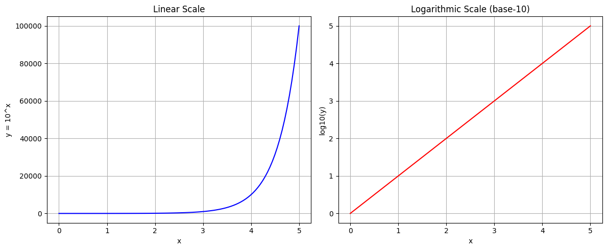
This "linearization" of an exponential process is a core benefit of logarithms. Consider an asset growing at a constant compounded rate. On a standard linear scale, its price follows an exponential curve. By taking the logarithm of the price, we transform this curve into a straight line, which is far simpler to analyze statistically.

This image illustrates how a logarithm transforms an exponential curve (left, linear scale) into a straight line (right, logarithmic scale). This is analogous to how log returns "straighten out" the analysis of compound growth in asset prices.

Calculating Log Returns in Python

As you're proficient in Python, let's translate this into code. The calculation is straightforward using the NumPy and Pandas libraries. You'll take the natural logarithm of the ratio of the current price to the previous day's price.

What Are Logarithmic Returns and How to Calculate Them in Pandas Dataframe | Saturn Cloud Blog

This blog post from Saturn Cloud provides a clear, finance-focused Python implementation.

First, review the definition for a quick recap. Then, focus on the section How to Calculate. Pay close attention to the use of np.log() for the logarithm and .shift(1) to access the previous day's price.

The core line of code you will use frequently is:

import numpy as np




# Assuming 'df' is a Pandas DataFrame with a 'Price' column
df['log_returns'] = np.log(df['Price'] / df['Price'].shift(1))

As noted in the article, the first value will be NaN (Not a Number) because there is no preceding price for the first data point. This is expected and is typically handled by dropping the first row before further analysis.

Conclusion

In this lesson, we've established the what, why, and how of logarithmic returns. They are the bedrock of quantitative financial analysis, and you will use them in almost every lesson that follows.

Here are the key takeaways:

Logarithmic returns represent continuously compounded returns and are derived from the mathematics of exponential growth using Euler's number, $e$ .
Their primary advantage is time-additivity, which allows you to sum returns over multiple periods, greatly simplifying analysis.
They possess more favorable statistical properties for modeling, as they tend towards a normal distribution, a core assumption in many financial models.
The calculation in Python is efficient and simple, using np.log() and the Pandas .shift() method.

Now that you understand how to calculate returns from a price series, our next step is to ensure that the price data itself is clean, accurate, and correctly formatted. In the next lesson, we will cover the critical procedures for performing data integrity checks and aligning time for intraday historical data feeds. This is a non-negotiable step before any reliable analysis can begin.

Recommended resources