In our last lesson, we explored the crucial metrics of drawdown and losing streaks, which quantify the "pain" a trading strategy can inflict. You now know how to measure the largest capital decline (maximum drawdown) and the longest run of losing trades. While essential, these risk metrics only tell one side of the story. To make informed decisions, we must view risk in the context of returns.
This lesson bridges that gap by introducing you to three of the most important risk-adjusted performance metrics in quantitative finance: the Sharpe, Sortino, and Calmar Ratios. You will learn how to calculate each one and, more importantly, understand what each ratio reveals about a strategy's performance. By the end, you'll be able to distill complex performance data into single, comparable figures that answer the fundamental question: "Am I being adequately compensated for the risk I'm taking?"
The Sharpe Ratio: The Industry Standard for Risk-Adjusted Return
The Sharpe Ratio is arguably the most widely used metric for comparing the performance of investments. Developed by Nobel laureate William F. Sharpe, it measures the excess return an investment generates per unit of total risk. "Excess return" is the return above a "risk-free" rate (like a government bond yield), and "total risk" is measured by the standard deviation of the returns (volatility).
The formula is:
Where:
- is the average return of the portfolio.
- is the risk-free rate of return.
- is the standard deviation of the portfolio's excess returns (its volatility).
Since returns data is often daily or monthly, the ratio is typically annualized to be comparable. For daily returns, you would multiply the average daily return by the number of trading days in a year (commonly 252 or 255) and the daily standard deviation by the square root of that same number.
The article "Sharpe, Sortino and Calmar Ratios with Python" from Codearmo provides a concise overview and Python implementation.
Sharpe, Sortino and Calmar Ratios with Python
This article offers clear definitions and Python code for the performance ratios we'll discuss. It's a great practical reference.
Please read the section on the Sharpe Ratio. Pay attention to the formula and how the Python function sharpe_ratio implements annualization by using the N parameter.
The Limitation of the Sharpe Ratio
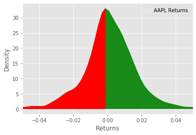
The Sharpe Ratio's simplicity is also its main weakness: it treats all volatility as "bad." Standard deviation measures the dispersion of returns around the mean, regardless of whether those returns are positive or negative. A strategy with large, positive outlier returns will have a higher volatility, which penalizes its Sharpe Ratio. This is counterintuitive, as traders welcome upside volatility. This flaw is especially apparent when analyzing strategies with skewed return distributions (i.e., not a perfect bell curve).
The Sortino Ratio: Focusing on "Bad" Volatility
The Sortino Ratio refines the Sharpe Ratio by addressing this very issue. It modifies the formula to only consider downside volatility—the volatility of negative returns. The rationale is simple: as an investor, you are primarily concerned with the risk of losing money, not the "risk" of making unexpectedly large gains.
Instead of standard deviation, the Sortino Ratio uses Target Downside Deviation (TDD), also known as downside deviation.
The formula is:
Where:
- is the average return of the portfolio.
- is the target rate of return, often set to 0 or the risk-free rate ().
- is the Target Downside Deviation.
The paper "Sortino: A 'Sharper' Ratio" provides an excellent and thorough explanation of the concept and its calculation. It's important to understand this correctly, as many online sources implement it improperly.
This document provides the definitive guide to understanding and correctly calculating the Sortino Ratio.
First, read the introduction on the Sharpe Ratio's limitations to solidify why a new metric was needed. Then, read the section on the Sortino Ratio itself. Most importantly, study the "Dissecting the Ratio" section to understand the mathematical definition of Target Downside Deviation (TDD). Finally, walk through the example calculation and the "Conclusion" which highlights common mistakes. Notice that returns above the target are not discarded; they are treated as zero deviation and included in the average, which is a crucial detail.
Now that you have the theory, let's look at the practical implementation in Python.
Sharpe, Sortino and Calmar Ratios with Python
This section of the Codearmo article provides the Python code to calculate the Sortino Ratio.
Read the Sortino Ratio section. The Python code here provides a simple, vectorized way to calculate downside deviation by filtering for negative returns (series[series<0]) before calculating the standard deviation. This is a common and practical implementation, assuming a target return of 0.
For two strategies with similar returns, the one with the higher Sortino Ratio achieves those returns with fewer and/or smaller losing periods.
The Calmar Ratio: A Drawdown-Based Perspective
While Sortino focuses on the volatility of losses, the Calmar Ratio takes a different approach. It directly measures return relative to the single worst experience: the maximum drawdown. This ratio is particularly useful for understanding if the strategy's overall return justifies the most significant capital loss it endured.
The formula is:
The Calmar Ratio is typically calculated over a 36-month period, but it's a valuable metric for any timeframe. It directly connects the reward (annual return) to the "pain" (max drawdown) you learned to calculate in the previous lesson. A higher Calmar Ratio is better, indicating strong returns relative to the worst-case loss.
Sharpe, Sortino and Calmar Ratios with Python
This final section from the Codearmo article covers the Calmar Ratio.
First, review the section on Max Drawdown as a refresher. Then, read the Calmar Ratio section to see the formula and its simple implementation in Python. Notice the use of abs() on the max drawdown, as it's conventionally expressed as a positive number in the ratio's denominator.
Automation with quantstats
Calculating these metrics manually is a great way to learn, but in practice, you'll want to automate this analysis. quantstats is a powerful Python library that does exactly that. With just a few lines of code, you can generate a comprehensive performance report, including all the ratios we've discussed and dozens more. This aligns perfectly with your goal of building a robust trading system.
The following video provides a fantastic overview of the library.
How to Backtest Trading Algorithms and Portfolio Metrics with Python and QuantStats
This video by Matt Macarty is a practical guide to using the quantstats library to analyze strategy performance and generate professional reports.
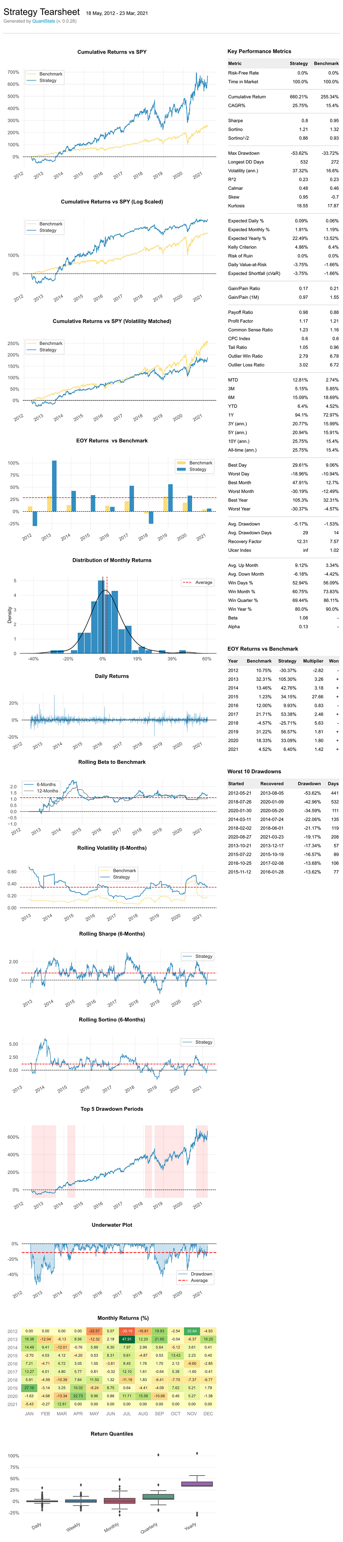
First, watch the section covering the stats module, which shows how to calculate individual metrics like the Sharpe Ratio and max drawdown. Then, watch the most powerful part of the video on the reports module. This demonstrates how a single command, qs.reports.html(), can generate a complete tearsheet comparing your strategy to a benchmark.
The output of quantstats is a professional-grade "tearsheet," like the one below. This is the kind of analysis you will eventually generate for your own strategies.
Conclusion
You have now added three essential risk-adjusted ratios to your quantitative toolkit. These metrics move beyond simple returns and provide a much richer, more nuanced view of a strategy's performance.
Here are the key takeaways:
- Sharpe Ratio: Measures excess return per unit of total volatility. It's the industry standard but penalizes for both upside and downside volatility.
- Sortino Ratio: An improvement on Sharpe, measuring excess return per unit of downside volatility only. It gives a better sense of reward versus "bad" risk.
- Calmar Ratio: Measures annualized return relative to the maximum drawdown. It directly assesses performance against the single worst period of capital loss.
- No Single Best Metric: Each ratio tells a different story. A thorough analysis involves looking at all of them to build a complete picture of a strategy's risk/reward profile.
In our next and final lesson of this introductory module, we will shift our focus from portfolio-level statistics to trade-level statistics by learning how to calculate a strategy's profit factor and expectancy. These metrics will help you understand the performance characteristics of your average trade.