Deterministic vs. Stochastic Sampling: A Practical Comparison

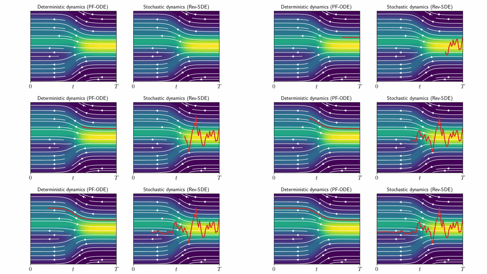
1. The ODE vs. SDE Perspective: Smooth Flow vs. Guided Random Walk

The core difference between deterministic and stochastic samplers can be understood by framing them as solvers for two different types of differential equations.

• Deterministic Samplers (like DDIM with $\eta =0$) are essentially solving an Ordinary Differential Equation (ODE). They follow a smooth, predictable vector field from a point in the noise space to a point on the data manifold (the space of realistic images).
• Stochastic Samplers (like DDPM) solve a Stochastic Differential Equation (SDE). They also follow a guiding vector field, but at each step, they add a small amount of random noise. This makes the path a "guided random walk."

This distinction is not just theoretical; it has direct visual consequences.

To build a stronger intuition, let's revisit the 2D spiral example.

As the video powerfully illustrates, the stochasticity in DDPM is not an arbitrary choice; it's a direct consequence of the underlying theory, preventing the model from collapsing to the mean of the learned distribution. DDIM provides a different theoretical path (the ODE) to arrive at the same target distribution without requiring this randomness, producing a sharp image deterministically.

2. Practical Consequences: Converging vs. Ancestral Samplers

In practice, this theoretical difference manifests in a very concrete way. Samplers are often categorized based on whether their output "converges."

• Converging Samplers (Deterministic): If you run the sampler with a fixed seed for 20 steps, and then run it again for 50 steps, the 50-step image will look like a more refined version of the 20-step image. The overall composition is fixed early on. Examples include DDIM and DPM++ 2M.
• Non-Converging / Ancestral Samplers (Stochastic): These samplers add noise at each step (hence "ancestral"). An image generated with 50 steps might look completely different from one generated with 20 steps, even with the same seed. Examples include Euler a and DPM++ 2S a. The 'a' often stands for "ancestral."

So, why have both?

• Deterministic Pros: Fast, reproducible, and enable features like DDIM inversion for image editing.
• Stochastic Pros: The added noise can act as a form of error correction. If the deterministic path (ODE) starts to veer off course early on, the error can amplify. The random "kick" from a stochastic sampler can nudge the trajectory back toward a more plausible region of the latent space, sometimes resulting in higher-quality images, especially at a low number of steps.

3. A Practical Experiment: Controlling Stochasticity

We can directly control the amount of stochasticity in many samplers. In DDIM, this is done with the eta ($\eta$) parameter we briefly mentioned last lesson.

• eta = 0: Fully deterministic DDIM.
• eta = 1: Fully stochastic, behaving like a DDPM sampler.
• 0 < eta < 1: A hybrid, semi-stochastic sampler.

This gives you a knob to turn, trading reproducibility for the potential error-correction benefits of noise. Let's see this in action.

This video provides the basis for a simple but powerful experiment you can run in any modern diffusion library like diffusers:

1. Select DDIM sampler with a fixed seed and prompt.
2. Set eta = 0.0. Generate an image with num_inference_steps=20, then another with num_inference_steps=50. Observe that the images are compositionally identical.
3. Now, set eta = 1.0. Keep the same seed and prompt. Generate again at 20 and 50 steps. Observe that the images are now completely different, demonstrating stochastic behavior.

This experiment directly shows the practical impact of moving between deterministic and stochastic strategies.

4. The Theory Behind the Knob: Churn and SDEs

The concept of injecting a controllable amount of noise is formalized in recent literature. Let's briefly connect our practical experiment back to the underlying theory.

This connects everything: the practical eta knob in your code is a direct implementation of the ${\eta }_t$ term in the formal stochastic differential equation. As an engineer, this gives you a solid theoretical grounding for your experimental choices. You're not just tweaking a random parameter; you're controlling the stochasticity of the differential equation solver.

Conclusion

In this lesson, we explored the crucial differences between deterministic and stochastic sampling strategies. We went beyond the simple "DDIM is fast" view to a more nuanced understanding of the trade-offs.

Key Takeaways:

• The ODE/SDE Spectrum: Deterministic samplers solve an ODE for a smooth, reproducible path, while stochastic samplers solve an SDE, following a guided random walk.
• Converging vs. Ancestral: Deterministic samplers converge to a final image composition early, while stochastic (ancestral) samplers change with each step.
• Error Correction vs. Speed: Stochasticity can help correct errors by "kicking" the sampler out of bad regions, but it comes at the cost of speed and reproducibility. Deterministic sampling is fast and reproducible but can amplify early errors.
• Practical Control: You can control this trade-off directly using parameters like eta (in DDIM) or by choosing samplers explicitly designed to be stochastic (those often ending in 'a').

Next Lesson Preview:

We've now covered the foundational sampling methods (DDPM, DDIM) and the principles of stochasticity. In the next lesson, we will build on this to explore a state-of-the-art family of samplers: DPM-Solvers. These are highly efficient ODE solvers that are now standard in many diffusion pipelines. We'll see how they provide excellent results in very few steps and how they also incorporate ideas like "churn" to get the best of both worlds.