Efficient Sampling with DPM-Solver

1. Beyond DDIM: The Power of High-Order Solvers

At its core, sampling in a diffusion model is about solving an ODE that transforms a noise vector ${\mathbf{x}}_T$ into a data sample ${\mathbf{x}}_0$. DDIM is a first-order solver, meaning it approximates the solution path using only the information at the current step. While a huge improvement over DDPM, it's still a relatively simple approximation.

Numerical methods for solving ODEs have a rich history, and it's well-known that higher-order solvers (like the Runge-Kutta methods you may have encountered) can achieve much higher accuracy for the same number of steps. DPM-Solver (Diffusion Probabilistic Model Solver) applies this principle, creating a family of high-order solvers specifically tailored to the structure of the diffusion ODE.

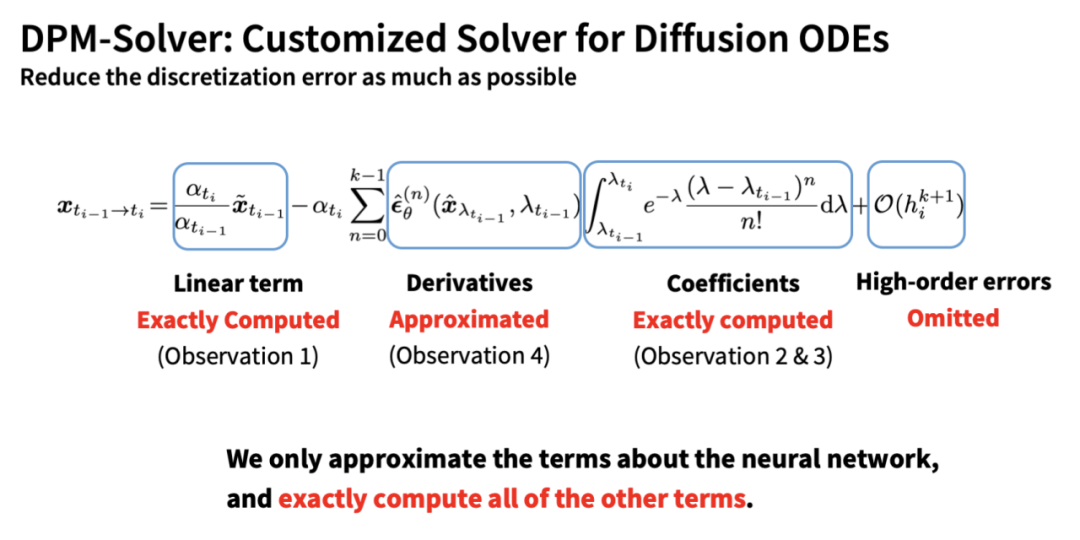
The key benefit is a dramatic increase in efficiency. Where DDIM might need 50, 100, or more steps for a high-quality result, DPM-Solvers can often achieve comparable or even better quality in just 15-25 steps.

2. DPM-Solver vs. DPM-Solver++: The Guided Sampling Problem

You'll encounter two main variants: DPM-Solver and DPM-Solver++. The distinction is critical for practical application, especially when using classifier-free guidance.

The original DPM-Solver, like other high-order methods, works well for unconditional sampling. However, researchers discovered a problem: when using strong classifier-free guidance, these solvers can become unstable and produce worse results than simple DDIM.

This is where DPM-Solver++ comes in.

This insight is crucial. DPM-Solver++ isn't just a minor update; it's a redesign specifically to handle the dynamics of guided sampling, which is the standard for most modern applications like text-to-image generation. As a result, for most of your work, DPM-Solver++ will be your default choice.

3. Practical Application with diffusers

Fortunately, using these advanced solvers is straightforward in libraries like Hugging Face diffusers. They are implemented as "schedulers" that you can easily swap into a pipeline.

The official DPM-Solver repository provides clear examples of this integration.

In diffusers, you'll primarily interact with these schedulers:

• DPMSolverMultistepScheduler: Implements the multistep variant.
• DPMSolverSinglestepScheduler: Implements the singlestep variant.
• DPMSolverSdeScheduler: A stochastic version, blending DPM-Solver with SDE principles.

The main distinction to understand is multistep vs. singlestep:

• Multistep: Uses the model's output from several previous timesteps to compute the next step. It's generally more accurate and stable, especially for guided sampling. This is the most commonly recommended variant.
• Singlestep: Only uses the information from the single most recent timestep. It's less memory-intensive and can be faster per-step, but might not achieve the same quality as the multistep version in the same number of total steps.

4. A Guide to Hyperparameter Tuning

Now for the most practical part: how do you configure the scheduler for the best results? Your goal as an engineer is to get the highest quality in the fewest steps. The DPM-Solver authors provide excellent, actionable recommendations.

Let's break down the key parameters you'll set when initializing the scheduler, using the guidance from the official repository.

Based on that reading, here is a summary of the most important parameters and the recommended heuristics:

1. algorithm_type: "dpmsolver" vs. "dpmsolver++"

   • As we learned, dpmsolver++ is designed for guided sampling and is generally the superior choice. Most modern pipelines default to this.

2. solver_order: 1, 2, or 3

   • This controls the order of the solver. solver_order=1 is equivalent to DDIM.
   • Heuristic:
     • For guided sampling (e.g., text-to-image with CFG), use solver_order=2. Higher orders can become unstable with guidance.
     • For unconditional sampling, you can use solver_order=3 for potentially higher quality.

3. use_karras_sigmas: True or False

   • This is a diffusers-specific parameter that uses a noise schedule proposed by Karras et al. (the "Elucidating the Design Space of Diffusion-Based Generative Models" paper). This schedule often improves detail and stability, especially at low step counts (under 30).
   • Heuristic: It's almost always a good idea to set this to True.

4. dynamic_thresholding: True or False

   • This is a technique to prevent pixel values from becoming saturated (too bright/dark) when using high guidance scales.
   • Crucial Caveat: This method is designed for pixel-space diffusion models (like Imagen). It is not suitable for latent-space models like Stable Diffusion, where the values in the latent space are not bounded in the same way. Applying it to Stable Diffusion can harm performance.
   • Heuristic: Leave this as False for latent diffusion models.

Putting it all together, a robust starting configuration for a Stable Diffusion pipeline would be:

from diffusers import StableDiffusionPipeline, DPMSolverMultistepScheduler
import torch

model_id = "stabilityai/stable-diffusion-2-1-base"

# 1. Initialize the scheduler with recommended settings
dpm_scheduler = DPMSolverMultistepScheduler.from_config(
    model_id,
    subfolder="scheduler",
    algorithm_type="dpmsolver++",
    solver_order=2,
    use_karras_sigmas=True
)

# 2. Load the pipeline with the custom scheduler
pipe = StableDiffusionPipeline.from_pretrained(
    model_id,
    scheduler=dpm_scheduler,
    torch_dtype=torch.float16
)
pipe = pipe.to("cuda")

# 3. Generate with a low number of steps
prompt = "a photorealistic portrait of an astronaut"
image = pipe(prompt, num_inference_steps=20).images[0]

This setup leverages the stability of dpmsolver++ with the recommended solver_order=2 for guidance and the improved karras_sigmas noise schedule, allowing for high-quality generation in just 20 steps.

Conclusion

In this lesson, we demystified the DPM-Solver family, one of the most significant advances in diffusion model sampling. You now have the practical knowledge to apply these solvers to accelerate your own pipelines significantly.

Key Takeaways:

• DPM-Solvers are high-order ODE solvers that can generate high-quality images in far fewer steps (15-25) than simpler methods like DDIM.
• DPM-Solver++ is the preferred variant for modern applications, as it was specifically designed to remain stable with classifier-free guidance.
• The multistep variant is generally recommended over the singlestep one for its accuracy and stability.
• You can tune DPM-Solvers with a few key heuristics:
  • Use algorithm_type="dpmsolver++".
  • Use solver_order=2 for guided sampling and solver_order=3 for unconditional.
  • Enable use_karras_sigmas=True for better low-step performance.
  • Only use dynamic_thresholding for pixel-space models.

Next Lesson Preview:

While a powerful solver like DPM-Solver is a huge piece of the puzzle, the final output quality is also deeply connected to the sequence of timesteps the solver operates on—the noise schedule. Different schedules can cause the solver to take larger or smaller steps in different parts of the denoising process. In our next lesson, we will learn how to debug sampling artifacts using noise schedule analysis, giving you another powerful tool for perfecting your model's output.