Ancestral Sampling with Noise Schedules

1. The Reverse Process: From Chaos to Order

The core idea of diffusion-based generation is to start with an image of pure, unstructured noise and progressively denoise it over hundreds or thousands of steps, guided by the trained U-Net model. This iterative reversal is what we call ancestral sampling.

To start, let's get a high-level intuition for this process.

As the video explained, each step in the reverse process, from a noisy image ${\mathbf{x}}_t$ to a slightly cleaner image ${\mathbf{x}}_{t-1}$, involves three key actions:

1. Denoise: Use the U-Net to predict the noise ${\mathbf{ϵ}}_{\theta }({\mathbf{x}}_t,t)$ and subtract a scaled version of it from the current image ${\mathbf{x}}_t$.
2. Correct Scale: Rescale the resulting image to account for the shrinking effect that occurred during the forward pass.
3. Inject Chaos: Add a small amount of new, random noise back into the image. This is the "ancestral" part of the name—each step has a stochastic component, creating a unique generation path.

The complete algorithm, as laid out in the original DDPM paper, is shown on the right side of the image below.

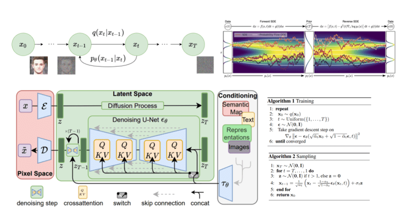
The formula for one step of this process (line 4 in Algorithm 2) is:

where $\mathbf{z}$ is new Gaussian noise, and ${\sigma }_t$ is the standard deviation of the noise added at this step. This equation is a direct implementation of the three intuitive steps we just discussed.

2. Implementing the Ancestral Sampling Loop

Now, let's translate this algorithm into code. Since you have a solid ML engineering background, we can go straight to a clean, well-annotated implementation.

The core of the logic resides in two functions:

1. A p_sample_loop function that initializes the process with random noise and iterates backward in time.
2. A p_sample function that executes the formula for a single denoising step.

Let's break down the key components from the reading:

• p_sample_loop(model, shape):

  • It starts by creating a tensor of pure Gaussian noise, img = torch.randn(shape, ...). This is our ${\mathbf{x}}_T$.
  • It then iterates from timesteps-1 down to 0. This is the reverse process.
  • In each iteration, it calls p_sample to get the slightly denoised image img for the next step.

• p_sample(model, x, t, t_index):

  • This function contains the core logic. It first extracts the necessary pre-calculated schedule values (${\beta }_t$, $\sqrt{1/{\alpha }_t}$, etc.) for the current timestep t.
  • It then computes the model_mean using the formula, which corresponds to the first term in the equation: $\frac{1}{\sqrt{{\alpha }_t}}({\mathbf{x}}_t-\frac{1-{\alpha }_t}{\sqrt{1-{\bar{\alpha }}_t}}{\mathbf{ϵ}}_{\theta }({\mathbf{x}}_t,t))$.
  • If t_index > 0, it samples new noise noise = torch.randn_like(x) and adds it, scaled by the posterior_variance_t. This is the "inject chaos" step.
  • If t_index == 0 (the final step), no new noise is added. We just return the mean.

For a more detailed, line-by-line walkthrough of a similar implementation, the following video is an excellent resource.

With these resources, you now have a complete picture of how ancestral sampling is implemented, from the high-level algorithm to the specific lines of PyTorch code.

3. The Noise Schedule: Architect of the Diffusion Process

We've mentioned the pre-calculated schedule values (${\alpha }_t$, ${\beta }_t$, etc.) several times. These are all derived from the noise schedule, ${\beta }_1,{\beta }_2,...,{\beta }_T$. This schedule is a fundamental hyperparameter that defines the entire diffusion process. It dictates how much noise is added at each forward step, which in turn determines the trajectory the model must learn to reverse.

The original DDPM paper used a simple linear schedule, where ${\beta }_t$ increases linearly from a small value to a larger one. However, subsequent research found that other schedules can lead to better results.

As you can see, swapping out a noise schedule is as simple as calling a different function to generate the betas tensor. Everything else in the sampling code remains the same.

But what is the practical difference between these schedules? A great way to visualize this is by plotting the Signal-to-Noise Ratio (SNR) over time. The SNR at timestep $t$ is defined as $\text{SNR}(t)={\bar{\alpha }}_t/(1-{\bar{\alpha }}_t)$. A high SNR means the signal (original image) dominates the noise, while a low SNR means the image is mostly noise.

From the plot, we can draw some key insights:

• Linear Schedule (Blue): The SNR drops relatively quickly and steadily. This means a significant amount of information is lost early in the forward process.
• Cosine Schedule (Orange): The SNR stays high for much longer and then drops more rapidly towards the end. This preserves more of the image structure during the initial forward steps. It has been empirically shown to improve sample quality. The intuition is that the model can spend more of its capacity on removing the last, most difficult bits of noise, rather than having to reconstruct coarse features that were destroyed too early.

The choice of schedule directly impacts the difficulty of the denoising task at each timestep t. A better-tuned schedule can make the learning problem easier for the U-Net and ultimately lead to higher-fidelity generated images.

Conclusion

In this lesson, we demystified the process of generating images with a diffusion model. We moved from the theory of training to the practice of sampling.

Key Takeaways:

• Ancestral sampling is the iterative, step-by-step process of reversing the forward diffusion process, starting from pure noise and ending with a clean image.
• Each sampling step involves using the trained U-Net to predict the noise, using that prediction to estimate a cleaner image, and injecting a small amount of new randomness to ensure sample diversity.
• The noise schedule (${\beta }_t$) is a critical set of hyperparameters that defines the noise level at each step. Its design significantly impacts model performance.
• Schedules like the cosine schedule often outperform the original linear schedule by preserving more signal throughout the forward process, leading to improved sample quality.
• Implementing different schedules is straightforward, typically involving swapping out a single function that generates the initial betas array.

Next Lesson Preview:

While ancestral sampling is effective, it is also slow, often requiring 1000 or more sequential model evaluations to generate a single image. This is a major practical limitation. In our next lesson, we will tackle this problem head-on by exploring a more advanced sampling method: Denoising Diffusion Implicit Models (DDIM). You will learn how DDIM generalizes the DDPM process and, most importantly, allows us to generate high-quality images in far fewer steps.