Diffusion Model Objectives

1. The Full ELBO vs. The Simplified Loss

Let's start with the conclusion from our last lesson. We found that minimizing the KL divergence between the model's reverse step and the true posterior simplifies to minimizing the squared error between the predicted and true noise:

This is the objective you likely implemented in your prior work. However, remember that this was a simplification. The full loss term derived directly from the ELBO contains a weighting factor that depends on the noise schedule:

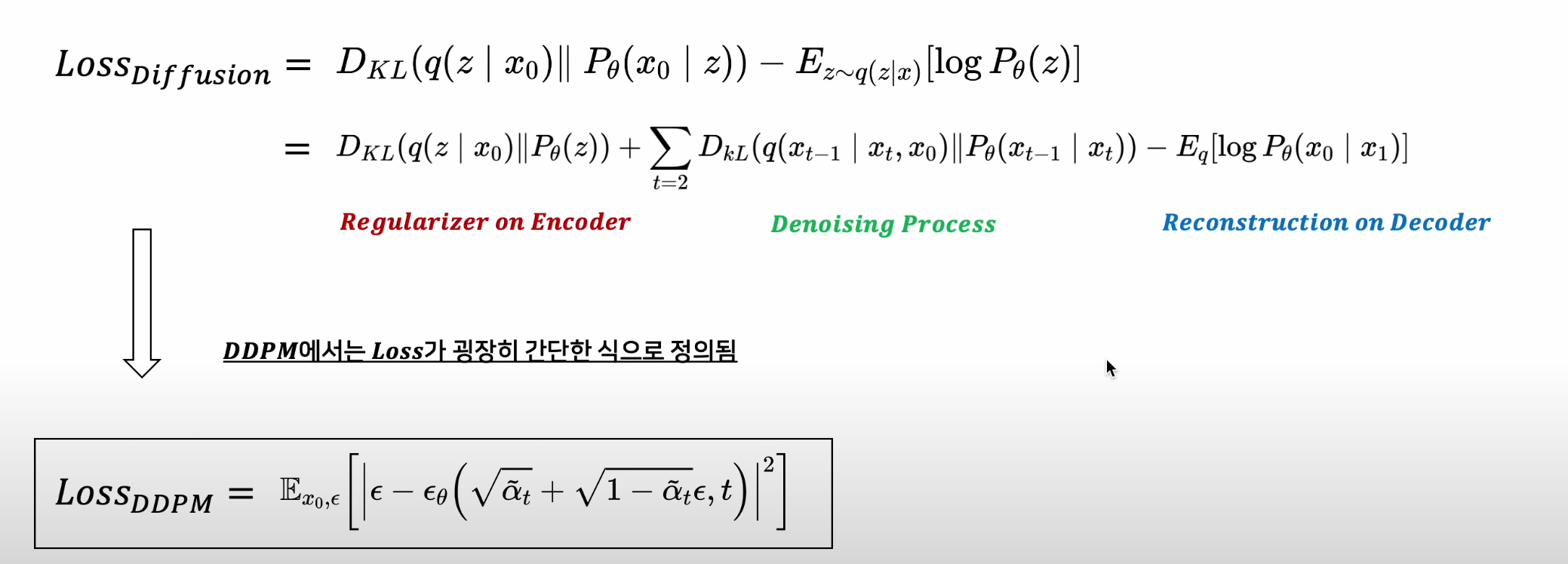
This distinction between the full, theoretically-derived ELBO loss and a simplified or re-weighted version is a central theme in modern diffusion models. While the ELBO provides a target for optimizing the data likelihood, practitioners often find that re-weighting the loss at different timesteps can yield better perceptual quality or training stability.

2. A Unified View of Prediction Targets

The choice of weighting is only one part of the story. The other is the choice of what the neural network, ${\mathbf{ϵ}}_{\theta }$, should predict. While predicting the noise $\mathbf{ϵ}$ is standard for DDPMs, it's not the only option. The model can be parameterized to predict other quantities, and the loss function can be adjusted accordingly.

The paper "Loss Functions in Diffusion Models: A Comparative Study" provides an excellent framework for unifying these different approaches. We'll use it as our guide.

As the paper outlines, we can re-parameterize our model and reformulate the loss to target different, but related, quantities. Let's look at each one.

A. $\mathbf{ϵ}$-space (Noise Prediction)

This is the familiar DDPM approach. The model ${\mathbf{ϵ}}_{\theta }({\mathbf{x}}_t,t)$ predicts the noise $\mathbf{ϵ}$ that was added to ${\mathbf{x}}_0$ to produce ${\mathbf{x}}_t$.

• Weighted Loss: $L_{ϵ}=||\mathbf{ϵ}-{\mathbf{ϵ}}_{\theta }({\mathbf{x}}_t,t)|{|}^2$
• Intuition: The network learns to "peel off" a layer of noise at each step. As noted in the paper LINK, this is a very stable and popular choice.

B. ${\mathbf{x}}_0$-space (Data Prediction)

Perhaps the most intuitive alternative is to have the model directly predict the clean image, ${\mathbf{x}}_0$, from the noisy input ${\mathbf{x}}_t$.

• Model: ${\mathbf{x}}_{0,\theta }({\mathbf{x}}_t,t)$
• Weighted Loss: $L_{x_0}=||{\mathbf{x}}_0-{\mathbf{x}}_{0,\theta }({\mathbf{x}}_t,t)|{|}^2$
• Intuition: At every step, the model tries to make its best guess of the final, clean image.

This is a very simple change from an implementation perspective. The blog post "Three Stable Diffusion Training Losses" provides a clear code-level view.

While simple, predicting ${\mathbf{x}}_0$ has a practical challenge. As $t\to T$, ${\mathbf{x}}_t$ becomes almost pure noise. The task of recovering ${\mathbf{x}}_0$ becomes extremely difficult, which can lead to high variance in the loss for later timesteps.

C. $\mathbf{s}$-space (Score Prediction)

This brings us back full circle to the score-matching foundation we discussed two lessons ago. The score, ${\nabla }_{{\mathbf{x}}_t}\log p_t({\mathbf{x}}_t)$, is the direction of steepest ascent in the log-probability of the noisy data distribution.

• Model: ${\mathbf{s}}_{\theta }({\mathbf{x}}_t,t)$
• Key Relationship: For Gaussian noise, the score is directly proportional to the noise: ${\nabla }_{{\mathbf{x}}_t}\log p_t({\mathbf{x}}_t,{\mathbf{x}}_0)=-\frac{\mathbf{ϵ}}{\sqrt{1-{\bar{\alpha }}_t}}$. This means predicting the score is equivalent to predicting a scaled version of the noise.
• Weighted Loss: $L_s=||{\nabla }_{{\mathbf{x}}_t}\log p_t({\mathbf{x}}_t)-{\mathbf{s}}_{\theta }({\mathbf{x}}_t,t)|{|}^2$
• Intuition: The model learns the vector field that points from noisy data towards regions of higher data density.

To see how score-matching objectives are constructed and optimized, this video provides an excellent deep dive.

This establishes that the DDPM framework can be seen as a specific implementation of a more general noise-conditional score-matching model.

D. $\mathbf{v}$-space (Velocity Prediction)

A more recent and highly effective formulation is $\mathbf{v}$-prediction, introduced in the paper "Progressive Distillation for Fast Sampling of Diffusion Models".

• Target: $\mathbf{v}=\sqrt{{\bar{\alpha }}_t}\mathbf{ϵ}-\sqrt{1-{\bar{\alpha }}_t}{\mathbf{x}}_0$
• Model: ${\mathbf{v}}_{\theta }({\mathbf{x}}_t,t)$
• Weighted Loss: $L_v=||\mathbf{v}-{\mathbf{v}}_{\theta }({\mathbf{x}}_t,t)|{|}^2$
• Intuition: The target $\mathbf{v}$ is a combination of the noise and the data. The name comes from an interpretation of the diffusion process as a particle moving along a path; $\mathbf{v}$ represents its velocity. A key benefit is that it has a unit-norm variance, making it well-behaved across all timesteps. It avoids the issues of ${\mathbf{x}}_0$-prediction at high noise and $\mathbf{ϵ}$-prediction at low noise, proving especially useful for model distillation and few-step sampling.

3. Comparing the Formulations: Theory vs. Practice

Now that we have these four different "spaces" (${\mathbf{x}}_0,\mathbf{ϵ},\mathbf{s},\mathbf{v}$), how do they compare?

Let's distill the key findings from that paper:

• Theoretical Equivalence: When using the full, un-simplified NELBO loss, all four formulations are mathematically equivalent. A perfect model trained on any of these NELBO losses would converge to the same solution.
• Practical Non-Equivalence: The simplified, un-weighted (or differently weighted) losses that are commonly used in practice are not equivalent. They place different emphasis on different timesteps.
• Likelihood vs. Sample Quality: Better likelihood (a lower NELBO loss) does not always correlate with better perceptual quality (e.g., lower FID score). For instance, the paper finds that $\mathbf{ϵ}$-space and $\mathbf{s}$-space achieve better likelihoods, but ${\mathbf{x}}_0$-space and $\mathbf{v}$-space can produce better samples.
• Behavior Across Timesteps:
  • ${\mathbf{x}}_0$-space loss is highest for large $t$ (high noise), as predicting the clean image from pure noise is very hard.
  • $\mathbf{ϵ}$-space loss is highest for small $t$ (low noise). Predicting a small noise vector requires high precision relative to the signal.
  • $\mathbf{v}$-space loss is more uniform across timesteps, which contributes to its training stability.

Conclusion

This lesson concludes our foundational module on diffusion theory. We've moved beyond the single DDPM objective to a more general understanding of the design choices available.

Key Takeaways:

• The standard DDPM training objective is a simplified, weighted loss where the model predicts the added noise ($\mathbf{ϵ}$).
• This is just one of four common formulations. The model can also be trained to predict the clean data (${\mathbf{x}}_0$), the score ($\mathbf{s}$), or a velocity term ($\mathbf{v}$).
• While the full NELBO-derived losses are theoretically equivalent, the simplified versions used in practice are not. They implicitly re-weight the objective, emphasizing different parts of the denoising process.
• The choice of prediction target is a practical one with significant trade-offs:
  • $\mathbf{ϵ}$-prediction is stable and works well.
  • ${\mathbf{x}}_0$-prediction is intuitive but can be unstable at high noise levels.
  • $\mathbf{s}$-prediction provides a direct link to score-based generative modeling.
  • $\mathbf{v}$-prediction offers improved stability and is particularly effective for few-step sampling and model distillation.

You now have a robust theoretical toolkit to understand, debug, and make informed decisions about the core training dynamics of diffusion models.

Next Lesson Preview:
Now that we have a solid understanding of how diffusion models are trained, we'll shift our focus to the other side of the process: inference and sampling. In the first lesson of our next module, "Advanced Sampling and Inference," we will implement the basic DDPM ancestral sampling algorithm and begin to explore how different choices, such as the noise schedule, can impact the speed and quality of the images we generate.