ELBO and DDPM Training

1. The Goal: Maximizing Log-Likelihood

As with many generative models, our ultimate goal is to train a model $p_{\theta }({\mathbf{x}}_0)$ that assigns high probability to samples from the true data distribution. We want to maximize the log-likelihood of our training data, ${\mathbb{E}}_{{\mathbf{x}}_0\sim p_{data}}[\log p_{\theta }({\mathbf{x}}_0)]$.

However, calculating $p_{\theta }({\mathbf{x}}_0)$ is intractable. It requires marginalizing over all possible latent paths from pure noise ${\mathbf{x}}_T$ back to the image ${\mathbf{x}}_0$:

This integral is over a very high-dimensional space, making direct optimization impossible.

2. The Solution: The Evidence Lower Bound (ELBO)

When a likelihood is intractable, a standard approach in machine learning is to optimize a tractable lower bound on it instead. For this, we use the Evidence Lower Bound (ELBO), also known as the Variational Lower Bound (VLB). You may recall this concept from your work with Variational Autoencoders (VAEs).

The core idea is to introduce the forward process distribution, $q({\mathbf{x}}_{1:T}|{\mathbf{x}}_0)$, and use Jensen's inequality to construct a lower bound on the log-likelihood.

The following short video provides a clear, animated derivation of how we arrive at the ELBO.

By maximizing this lower bound, L_VLB, we push up the true log-likelihood log p_theta(x_0).

3. Deconstructing the ELBO

The raw form of the ELBO isn't very practical for training. The key insight in the DDPM paper is to rewrite it as a sum of more interpretable terms. After applying Bayes' theorem and exploiting the Markov property of the forward and reverse chains, the ELBO can be expressed as:

This can be re-written as a sum of KL divergences, which gives us a clearer picture of what the model is learning at each stage.

Let's summarize the three key components from that reading:

1. Reconstruction Term ($L_0$): ${\mathbb{E}}_q[\log p_{\theta }({\mathbf{x}}_0|{\mathbf{x}}_1)]$. This is like the decoder in a VAE, measuring how well the model can reconstruct the original image ${\mathbf{x}}_0$ from the first-step latent ${\mathbf{x}}_1$.
2. Prior Matching Term ($L_T$): $D_{KL}(q({\mathbf{x}}_T|{\mathbf{x}}_0)||p({\mathbf{x}}_T))$. This measures how well the distribution of the final noisy latent ${\mathbf{x}}_T$ (from the forward process) matches our chosen prior, which is typically a standard normal distribution. Since the forward process is designed to produce a standard normal distribution at time $T$, this term is close to zero and has no trainable parameters, so it's often ignored during training.
3. Denoising Matching Term ($L_{t-1}$ for $t\in [2,T]$): $D_{KL}(q({\mathbf{x}}_{t-1}|{\mathbf{x}}_t,{\mathbf{x}}_0)||p_{\theta }({\mathbf{x}}_{t-1}|{\mathbf{x}}_t))$. This is the heart of the training process. For each step, it forces our learned reverse transition $p_{\theta }$ to match the true reverse transition $q$.

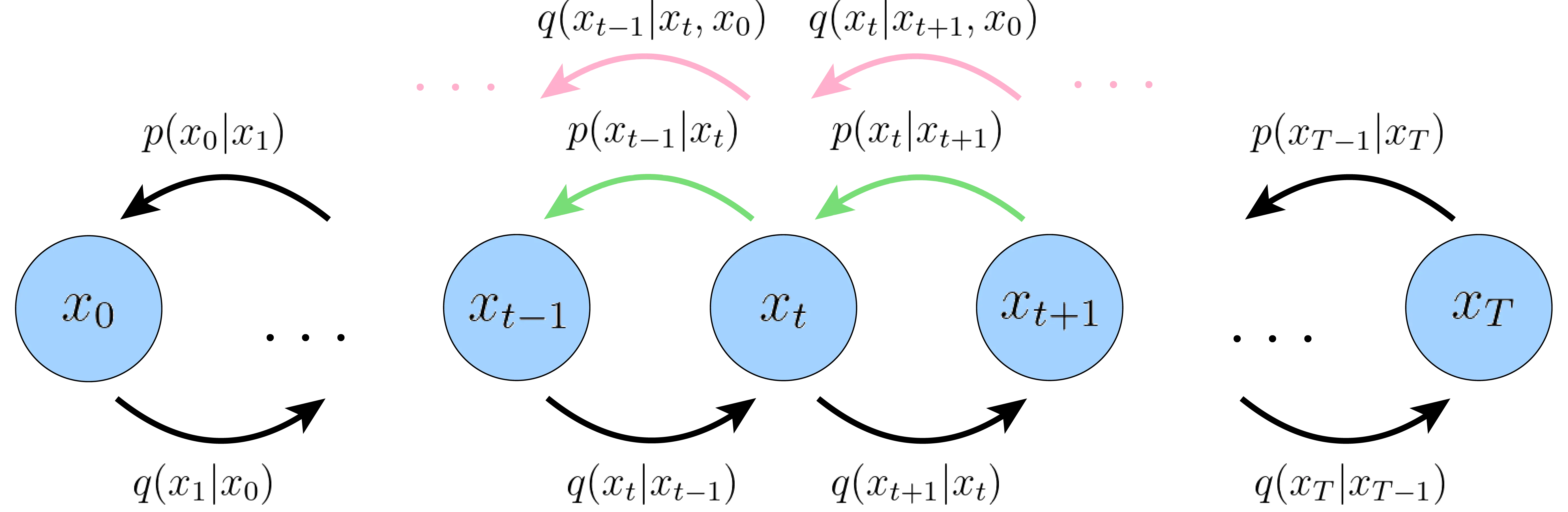
4. Simplifying the Denoising Term

The Denoising Matching Term looks problematic because our model $p_{\theta }({\mathbf{x}}_{t-1}|{\mathbf{x}}_t)$ doesn't get to see the original image ${\mathbf{x}}_0$, while the target distribution $q({\mathbf{x}}_{t-1}|{\mathbf{x}}_t,{\mathbf{x}}_0)$ does. This is not a problem; in fact, it's the core of the supervision. We are training the model to approximate this "cheating" posterior, but without cheating.

The true posterior $q({\mathbf{x}}_{t-1}|{\mathbf{x}}_t,{\mathbf{x}}_0)$ is a Gaussian whose parameters (mean ${\tilde{\mathbf{\mu }}}_t({\mathbf{x}}_t,{\mathbf{x}}_0)$ and variance ${\tilde{\beta }}_t$) can be calculated in closed form because we know everything about the forward process.

Our model's reverse transition, $p_{\theta }({\mathbf{x}}_{t-1}|{\mathbf{x}}_t)$, is also parameterized as a Gaussian, with a learned mean ${\mathbf{\mu }}_{\theta }({\mathbf{x}}_t,t)$ and a variance ${\mathbf{\Sigma }}_{\theta }({\mathbf{x}}_t,t)$.

The DDPM paper makes a crucial simplification: they fix the variance ${\mathbf{\Sigma }}_{\theta }$ to be a non-learned constant (e.g., ${\tilde{\beta }}_t$). The KL divergence between two Gaussians with the same variance simplifies to the squared L2 distance between their means, scaled by the variance.

This transforms the problem: the neural network's only job is to predict the correct mean for the denoising step.

5. From Predicting the Mean to Predicting the Noise

We're almost there. The final step is a reparameterization that makes the objective even simpler. The true mean ${\tilde{\mathbf{\mu }}}_t$ is a somewhat complex function of ${\mathbf{x}}_t$ and ${\mathbf{x}}_0$. The key idea is to express both the true mean and the predicted mean in terms of the noise $\mathbf{ϵ}$ that was added at step $t$.

The following video shows this final, elegant step.

As the video explains, by parameterizing our model to predict the noise ${\mathbf{ϵ}}_{\theta }({\mathbf{x}}_t,t)$, the loss term becomes:

This is exactly the simple Mean Squared Error objective we arrived at from the score-matching perspective! The authors of the DDPM paper found that ignoring the weighting factors and using this simple loss worked best in practice.

The Complete Training Algorithm

This derivation leads directly to the training algorithm outlined in the DDPM paper. The resource we looked at earlier provides a concise summary.

This simple loop is the foundation of DDPM training and is what you would have implemented in your prior experience. You now have a complete theoretical picture of its justification from a variational inference standpoint.

Conclusion

In this lesson, we dug into the theoretical underpinnings of the DDPM training objective from a variational inference perspective.

Key Takeaways:

• The DDPM training objective is derived by maximizing the Evidence Lower Bound (ELBO) on the data log-likelihood.
• The ELBO can be decomposed into terms representing reconstruction, prior matching, and denoising matching.
• The crucial denoising matching term minimizes the KL divergence between the model's reverse transition and the true (but "cheating") posterior, $q({\mathbf{x}}_{t-1}|{\mathbf{x}}_t,{\mathbf{x}}_0)$.
• By fixing the variance of the reverse process, this objective simplifies to minimizing the L2 distance between the true and predicted means of the denoising steps.
• A final reparameterization trick elegantly transforms the mean-matching objective into a simple Mean Squared Error between the true noise $\mathbf{ϵ}$ and the predicted noise ${\mathbf{ϵ}}_{\theta }$.
• This result provides a powerful, alternative justification for the same simple loss function we derived from score-matching, solidifying its theoretical grounding.

In our next lesson, we will wrap up our foundational theory module by analyzing and comparing different formulations of this training objective. We'll discuss the practical differences between the simplified MSE loss and the full variational bound, and briefly introduce alternative prediction targets like predicting ${\mathbf{x}}_0$ directly.