Score Distillation Sampling Explained

Hello and welcome to the next phase of your journey into diffusion models.

In the previous module, you mastered the fundamentals of Neural Radiance Fields (NeRFs), culminating in the implementation of the volume rendering equation. You now have a complete, differentiable pipeline to render a 2D image from a 3D NeRF representation.

This lesson marks a pivotal transition. We will now connect your expertise in 3D rendering with the power of diffusion models to tackle one of the most exciting areas of generative AI: text-to-3D generation. Our goal for this lesson is to explain the core mechanism of Score Distillation Sampling (SDS) for guiding a 3D representation with a 2D diffusion model. This is the foundational technique that underpins models like Google's DreamFusion.

1. The Big Idea: A 2D Diffusion Model as a 3D Critic

Imagine you have a randomly initialized NeRF. It produces a blob-like, colorless 3D shape. How can you optimize the weights of this NeRF so it represents, for example, "a DSLR photo of a peacock on a surfboard"?

The primary challenge is the lack of data. We don't have large-scale datasets of high-quality 3D models paired with text descriptions. However, we do have incredibly powerful pre-trained 2D text-to-image diffusion models (like Imagen or Stable Diffusion) that have learned a deep semantic understanding of the relationship between text and images.

Score Distillation Sampling (SDS) provides the bridge. The core idea is to use one of these powerful 2D models as a "critic" or a "loss function" that can guide the optimization of a 3D model's parameters.

The process works in a loop:

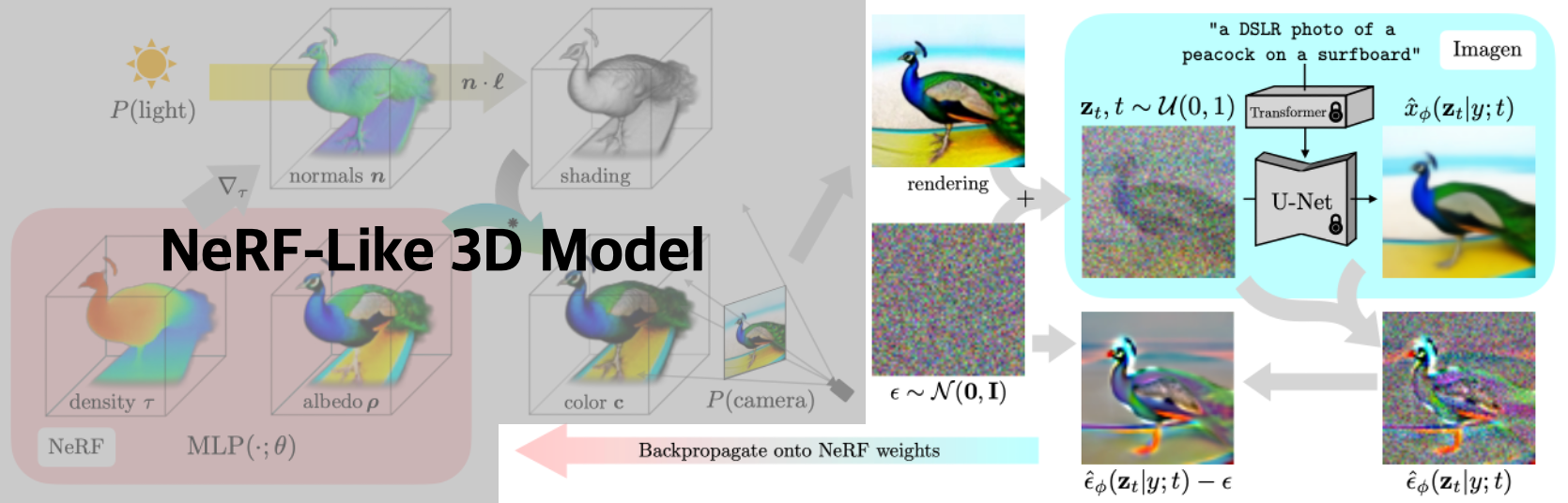
Render: Pick a random camera angle and render a 2D image of your current 3D NeRF. This step is fully differentiable, thanks to the work you did in the last module.
Evaluate: Pass this rendered image to a pre-trained 2D text-to-image diffusion model. The model assesses how well the image matches the target text prompt.
Update: Use the feedback from the diffusion model to calculate a gradient. Backpropagate this gradient through the differentiable renderer to update the weights of the NeRF.

By repeating this process with thousands of different camera angles, the NeRF is gradually "sculpted" to look correct from every viewpoint, effectively creating a coherent 3D object that matches the text prompt.

The diagram below, from the DreamFusion paper, illustrates this entire pipeline beautifully.

Score Distillation Sampling (SDS) for Text-to-3D Generation — This diagram shows the complete SDS loop. A 3D NeRF (left) is rendered into a 2D image. This image is then evaluated by a pre-trained 2D diffusion model (right) against a text prompt. The resulting error signal (gradient) is backpropagated to update the NeRF's weights, progressively refining the 3D model.

2. The "Distillation" Trick: Why Not Just Use the Diffusion Loss?

Given your ML background, a natural first thought might be to use the standard diffusion model training objective as the loss. That is, for a rendered image $x$ , we could:

Add noise to get $x_{t}$ .
Predict the noise with the diffusion model: $ϵ_{θ} (x_{t}, y, t)$ .
Compute the MSE loss: $∣∣ ϵ - ϵ_{θ} (x_{t}, y, t) ∣ ∣^{2}$ .
Backpropagate the gradient of this loss to update the NeRF parameters.

It turns out this naive approach doesn't work well. A great blog post by Sander Dieleman explains why.

The paradox of diffusion distillation

The blog post 'The paradox of diffusion distillation' provides a concise explanation of the problem with the naive approach and the key insight behind SDS.

Read the section starting with 'Naively, one could think...' It's short but contains the crucial insight. Focus on the role of the 'Jacobian of the diffusion model' and the solution SDS proposes.

As the post highlights, the problem lies in the gradient. Backpropagating through the full diffusion loss involves the Jacobian of the diffusion model's U-Net, which is noisy and poorly conditioned, leading to poor optimization.

The key innovation of SDS is to cleverly reformulate the gradient to avoid this. Instead of backpropagating through the diffusion model, we treat the model's output as a fixed target. We only need to perform a forward pass to get the noise prediction.

The resulting "pseudo-gradient" provides a direction for updating the NeRF's parameters $ϕ$ :

\nabla_{ϕ} L_{S D S} (ϕ) = E_{t, ϵ} [w (t) (ϵ_{θ} (x_{t}, y, t) - ϵ) \frac{\partial x}{\partial ϕ}]

Let's break this down:

$ϵ_{θ} (x_{t}, y, t)$ is the noise predicted by the diffusion model.
$ϵ$ is the actual noise we added to the rendered image $x$ .
$(ϵ_{θ} - ϵ)$ is the "error" term. It represents the update direction that would make the noisy image $x_{t}$ more plausible according to the diffusion model.
$\frac{\partial x}{\partial ϕ}$ is the Jacobian of our renderer, which chains the gradient back to the NeRF parameters $ϕ$ .
$w (t)$ is a weighting function that depends on the timestep, typically down-weighting timesteps with very high or very low noise.

Essentially, we're using the diffusion model to predict the "denoising direction" and applying that direction as an update to our NeRF. This is why it's called "distillation"—we are distilling the score (gradient of the log-probability) of the powerful 2D diffusion model into our 3D representation.

The image below contrasts standard diffusion sampling (which updates pixels) with SDS (which updates generator parameters).

Comparison of Ancestral Sampling and Score Distillation Sampling — Comparison of standard ancestral sampling (left), where pixel values are iteratively updated, and Score Distillation Sampling (right), where the parameters $\theta$ of a generator $g$ are updated by minimizing a loss derived from the diffusion model's score.

3. The Role of Classifier-Free Guidance (CFG)

To get high-quality results that strongly align with the text prompt, SDS heavily relies on Classifier-Free Guidance (CFG), a technique you'll be familiar with from 2D diffusion. The implementation is analogous to how it's used in standard image generation.

We compute two noise predictions:

Conditional: $ϵ_{θ} (x_{t}, y, t)$ , using the target text prompt $y$ .
Unconditional: $ϵ_{θ} (x_{t}, \emptyset, t)$ , using an empty or generic prompt.

The final noise prediction used for the gradient calculation is a guided combination:

ϵ^_{θ} = ϵ_{θ} (x_{t}, \emptyset, t) + ω \cdot (ϵ_{θ} (x_{t}, y, t) - ϵ_{θ} (x_{t}, \emptyset, t))

Here, $ω$ is the guidance scale. The SDS gradient then becomes:

\nabla_{ϕ} L_{S D S} (ϕ) \propto (ϵ^_{θ} - ϵ) \frac{\partial x}{\partial ϕ}

This guided update pushes the NeRF parameters $ϕ$ in a direction that strongly emphasizes the prompt's content. For a detailed guide on how this is implemented in practice, the following resource is excellent.

3D Gaussian Splatting and Diffusion Guided Optimization

This guide from a university assignment on 3D deep learning provides a clear, step-by-step walkthrough for implementing the SDS loss, including the CFG component.

Read section '2.1 SDS Loss + Image Optimization'. Focus on the two implementation steps: 'SDS without guidance' and 'SDS with guidance'. This directly explains how the theoretical gradient is translated into a practical loss function for a PyTorch training loop.

As noted in the resource, CFG is essential for good results. DreamFusion found that using a very high guidance scale ( $ω = 100$ ) was beneficial. This relates to the "mode-seeking" nature of the SDS loss, which aggressively optimizes for a high-probability output under the diffusion model's distribution. This can sometimes lead to artifacts like oversaturation, but it is highly effective at creating a single, coherent object.

Test your understanding!

In the SDS update step, we calculate the gradient that updates our NeRF's weights. Why do we not need to backpropagate through the U-Net of the 2D diffusion model? What is the practical engineering benefit of this?

Show answer

We don't need to backpropagate through the U-Net because the SDS gradient formulation, $\nabla_{ϕ} L_{S D S} \propto (ϵ^_{θ} - ϵ) \frac{\partial x}{\partial ϕ}$ , treats the predicted noise $ϵ^_{θ}$ as a fixed target for a given step. The gradient calculation only requires the output of a forward pass through the U-Net, not the intermediate activations.

The practical engineering benefit is enormous. Pre-trained text-to-image models like Stable Diffusion have billions of parameters. Avoiding backpropagation through this massive network dramatically reduces memory consumption and computational complexity. We only need to backpropagate through our much smaller, differentiable renderer and the NeRF MLP. This makes text-to-3D optimization feasible on consumer-grade hardware.

Conclusion

In this lesson, you've learned the core mechanism of Score Distillation Sampling (SDS), the conceptual bridge that allows us to use 2D generative models to create 3D assets.

Key Takeaways:

SDS leverages a pre-trained 2D text-to-image diffusion model as a "critic" to optimize a 3D representation (like a NeRF) from a text prompt, without requiring any 3D training data.
The optimization happens in a loop: render a 2D view, get feedback from the 2D model, and backpropagate a gradient to the 3D model's parameters.
The core "trick" of SDS is its specialized gradient formulation. It avoids backpropagating through the massive diffusion U-Net by treating its noise prediction as a fixed value, which circumvents issues with unstable Jacobians and dramatically reduces computational cost.
Classifier-Free Guidance (CFG) is used with a high guidance scale to steer the optimization strongly towards the text prompt, which is crucial for generating coherent and detailed objects.

Next Lesson Preview:

Now that you understand the theory behind the SDS gradient, we will begin putting the pieces together for a full implementation. In the next lesson, you will implement the first part of the text-to-3D training loop: rendering a 2D view from a 3D representation at a random camera angle. While you've implemented rendering before, we'll now focus on the strategy of camera sampling, which is critical for ensuring the 3D object is optimized coherently from all sides.

Recommended resources

1. The Big Idea: A 2D Diffusion Model as a 3D Critic

2. The "Distillation" Trick: Why Not Just Use the Diffusion Loss?

3. The Role of Classifier-Free Guidance (CFG)

Conclusion