2D View Generation from 3D Representations

1. The Camera Model: From a Pose to Rays

To render a 2D view, we first need to define "where" we are looking from. In computer graphics and robotics, a camera's position and orientation in 3D space (its "pose") is typically encapsulated in a 4x4 camera-to-world (c2w) transformation matrix.

This matrix efficiently combines two operations:

• A 3x3 rotation matrix that defines the camera's orientation.
• A 3x1 translation vector that defines the camera's position (origin) in world coordinates.

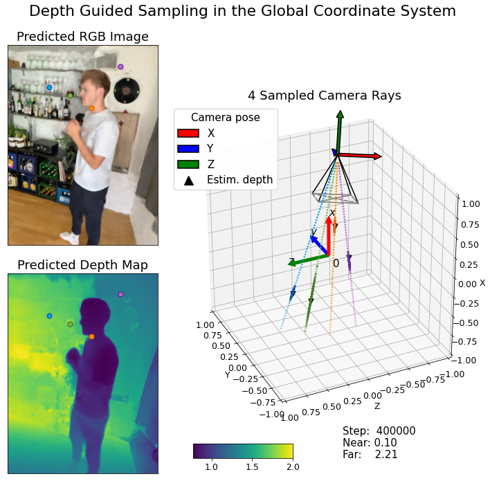
The next step is to use this pose to generate the set of rays needed for rendering. We do this using a pinhole camera model. For each pixel in our desired output image (e.g., a 256x256 image), we calculate the origin and direction of a ray that starts at the camera's center and passes through that specific pixel.

The following Google Colab notebook provides a very clear, practical implementation of this process.

Let's break down the logic of the get_rays function you just reviewed:

1. Pixel Coordinates: It first creates a grid of (i, j) pixel coordinates.
2. Camera-Space Directions: It converts these pixel coordinates into direction vectors in the camera's local coordinate system. This step uses the focal_length to determine the field of view and centers the coordinates. The z component is typically set to -1, indicating that the camera looks along its negative z-axis.
3. World-Space Transformation: It then transforms these camera-space direction vectors into the world coordinate system.
   • The rays_d (directions) are calculated by multiplying the camera-space directions with the rotation part of the c2w matrix (c2w[:3, :3]).
   • The rays_o (origins) are the same for every ray: they are simply the camera's position, which is the translation part of the c2w matrix (c2w[:3, -1]).

For the SDS loop, we will repeatedly call this function, feeding it a randomly sampled c2w matrix each time to ensure our 3D model is optimized from all angles.

2. From Rays to Pixels: Volume Rendering

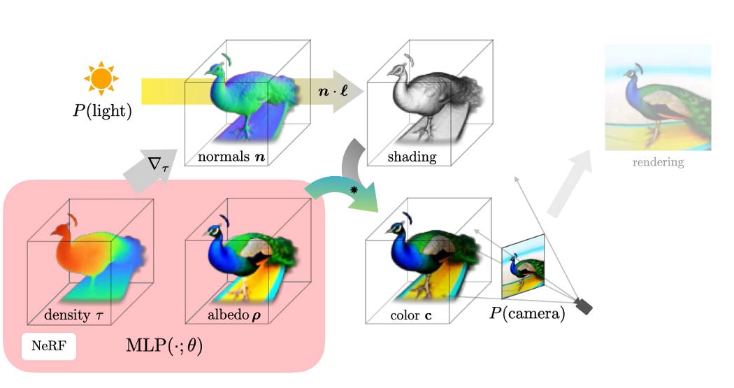
Once we have the origin and direction for every ray, we can render the final image using the volume rendering technique you're familiar with from Module 8. As a quick refresher, this involves:

1. Sampling: Taking a number of sample points along each ray.
2. Querying: Feeding the 3D coordinates of these points into our NeRF's MLP to get a color $\mathbf{c}$ and a volume density $\sigma$ for each point.
3. Compositing: Accumulating these colors and densities along the ray to calculate the final pixel color, using the discrete volume rendering equation:
   $\hat{C}(\mathbf{r})={\sum }_{i=1}^N{T}_i{\alpha }_i{\mathbf{c}}_i\text{where}{T}_i={\prod }_{j=1}^{i-1}(1-{\alpha }_j)\text{and}{\alpha }_i=1-\exp (-{\sigma }_i{\delta }_i)$

To see how this is implemented in code, the following video provides a clear, step-by-step walkthrough.

The video you just watched and the Colab notebook from earlier (LINK, section "Volume Rendering") both implement this process. The core steps are:

• Stratified Sampling: Instead of just taking uniformly spaced points, a small random perturbation is added to the samples within each interval. This helps the model learn a continuous representation rather than overfitting to specific discrete locations.
• Calculating alpha and weights: The predicted densities ($\sigma$) and the distances between samples ($\delta$) are used to compute the opacity ($\alpha$) of each sample. These are then used to compute the transmittance ($T$) and the final color weight for each sample point.
• Weighted Sum: The final pixel color (rgb_map) is a weighted sum of the colors (${\mathbf{c}}_i$) of all samples along that ray, using the computed weights.

3. Assembling the Full Rendering Pipeline

We now have all the necessary components. We can combine them into a single function that takes a camera pose and a NeRF model, and returns a rendered 2D image.

The nerf_forward function in the "NeRF From Nothing" Colab notebook (LINK, section Hierarchical Volume Sampling) serves as a perfect example of such a pipeline. It encapsulates the entire process:

1. It takes rays_o and rays_d as input. (These would be generated by our get_rays function using a specific camera pose).
2. It performs stratified sampling to get query points (query_points).
3. It runs these points through the NeRF model (coarse_model).
4. It calls raw2outputs to perform volume rendering and produce an rgb_map.
5. (Optionally, it performs hierarchical sampling for a fine pass, which improves detail but follows the same principles).

In the context of our text-to-3D goal, our training loop will look something like this for each step:

# 1. Sample a random camera pose
random_pose = sample_random_camera_pose() # e.g., on a hemisphere

# 2. Generate rays for this pose
rays_o, rays_d = get_rays(height, width, focal, random_pose)

# 3. Render the 2D image using the current NeRF
# This function encapsulates sampling, querying the NeRF, and volume rendering
outputs = nerf_forward(rays_o, rays_d, nerf_model)
rendered_image = outputs['rgb_map']

# 4. Use the rendered_image in the SDS loss calculation (Next Lesson!)
# ...

This lesson has focused on implementing steps 2 and 3. You are now equipped with the practical knowledge to generate the 2D views that form the input to the SDS loss.

Conclusion

In this lesson, you've translated the rendering requirement of the SDS pipeline into a concrete implementation plan. You now understand how to go from an abstract camera pose to a fully rendered 2D image of a NeRF.

Key Takeaways:

• A camera's position and orientation are defined by a 4x4 camera-to-world (c2w) matrix.
• The get_rays function uses the pinhole camera model to convert a c2w matrix into a unique origin and direction vector for each pixel of the desired image.
• Volume rendering synthesizes the final pixel color by sampling points along each ray, querying the NeRF for color and density, and composing them using a weighted sum based on opacity and transmittance.
• The entire rendering pipeline is differentiable, allowing gradients from a 2D loss function to flow back and update the 3D NeRF's parameters.

Next Lesson Preview:

You've built the function that generates the input for our 2D diffusion critic. In the next lesson, we will implement the other side of the equation: the SDS loss function. You will learn how to take the rendered image, add noise, pass it to a pre-trained 2D diffusion model, and calculate the special SDS gradient that will be used to optimize our NeRF.