SDS Loss for Single-View Diffusion Models

1. The Core Idea: Why Not Just Use a Standard Diffusion Loss?

Let's say we have our rendered image x from the NeRF and a text prompt y. A natural first thought might be to use a standard diffusion model training objective:

1. Add noise to x to get a noisy image x_t.
2. Ask the diffusion model ε_θ to predict the noise ε_pred = ε_θ(x_t, y, t).
3. Calculate the mean squared error: L = ||ε_pred - ε||².
4. Backpropagate this loss to update the NeRF parameters θ.

The problem lies in step 4. To compute the gradient ∂L/∂θ, the chain rule requires us to compute ∂L/∂x, which means backpropagating through the entire diffusion model's U-Net (ε_θ). As you know from your ML engineering background, this is computationally prohibitive and can be numerically unstable, especially since the U-Net wasn't trained to have well-behaved gradients with respect to its input image.

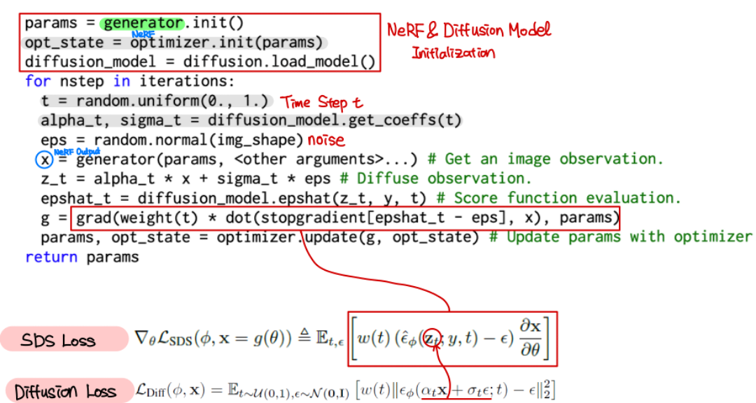
Score Distillation Sampling provides an elegant and efficient solution. It computes a gradient that pushes x towards a region of higher probability according to the diffusion model, but does so without requiring gradients to flow back through the U-Net.

2. The Score Distillation Sampling (SDS) Gradient

The goal of SDS is to find a gradient ∇_θ L that we can use with an optimizer to update our NeRF's parameters θ. The derivation in the original DreamFusion paper shows that this gradient can be formulated as:

Let's break down this equation:

• x = g(θ) is our rendered image from the NeRF.
• x_t = α_t x + σ_t ε is the noisy image at timestep t.
• ε_φ(x_t; y, t) is the noise prediction from our pre-trained 2D diffusion model ε_φ.
• (ε_φ - ε) is the crucial distillation signal. It's the difference between the predicted noise and the actual noise. This vector tells us how to modify x_t to make it look more like a sample the diffusion model would expect.
• w(t) is a weighting function that depends on the timestep. It modulates the strength of the gradient. The DreamFusion paper found that a simple uniform weighting (w(t)=1) works well.
• ∂x/∂θ is the Jacobian of our NeRF renderer. It translates the "image-space" update direction into a gradient for the NeRF's parameters θ. The beauty of modern ML frameworks like PyTorch is that autograd handles this for us automatically.

The key insight is how this is implemented. We treat the noise prediction ε_φ as a fixed constant for the backward pass. We compute it in a forward pass, and then detach() it from the computation graph before using it to define our gradient.

3. Implementing the SDS Loss Function

Now, let's turn theory into practice. Your task is to implement the loss calculation. We will follow the structure of a practical programming assignment, which will prepare you for real-world implementation.

As described in the resource, the get_sds_loss() function in guidance/sd.py takes the rendered image (which they call latent_image because it's often done in the VAE's latent space, but for now we can think of it as our x), and the text embedding c. Here is the step-by-step process to implement it:

1. Sample Timestep t: The theory integrates over all t, but in practice, we sample a single t for each training step. The DreamFusion paper suggests sampling uniformly from a range that avoids the extremes, like t ~ U(0.02, 0.98), to prevent numerical instability.

   # t is typically an integer from 0 to T-1
   t = torch.randint(int(T * 0.02), int(T * 0.98), (batch_size,), device=device)
   

2. Add Noise (Forward Process): Use the t and a random noise sample ε to create the noisy image x_t. You'll need the noise schedule's alphas_cumprod to get the correct α_t and σ_t for the forward process formula you know well.

   # Sample random noise
   noise = torch.randn_like(latents)
   
   # Add noise to the latents to get x_t
   noisy_latents = scheduler.add_noise(latents, noise, t)
   

3. Predict Noise with CFG: This is a critical step. To get a strong signal, we use Classifier-Free Guidance (CFG).

   • Run the U-Net twice: once with the text prompt embedding c and once with a null-text embedding c_null.
   • Combine the predictions: ε_pred = ε_pred_uncond + guidance_scale * (ε_pred_text - ε_pred_uncond).
   • The DreamFusion paper notes that a very high guidance_scale (e.g., 100) is often necessary for SDS to prevent overly smooth or averaged-out results.

   # Predict the noise for both conditional and unconditional offerings
   noise_pred_text = unet(noisy_latents, t, encoder_hidden_states=text_embeddings).sample
   noise_pred_uncond = unet(noisy_latents, t, encoder_hidden_states=null_embeddings).sample
   
   # Perform CFG
   noise_pred = noise_pred_uncond + guidance_scale * (noise_pred_text - noise_pred_uncond)
   

4. Calculate the SDS Gradient: As per the formula, the gradient direction is simply the difference between the predicted noise and the actual noise. We also apply the w(t) weighting, which for simplicity is often set to 1 or tied to the noise schedule.

   # Can be w(t) = 1 or a function of the scheduler's sigmas
   w_t = 1.0 
   grad = w_t * (noise_pred - noise)
   

5. Define the Loss for Backpropagation: Here's the implementation trick. The KAIST assignment asks for a scalar loss to be returned, which is standard in most training loops. We need to define a loss L such that its gradient with respect to our input x (latents) is the grad we just calculated.

   A common and effective way to achieve this is to use the backward() method with a gradient argument. You can define a dummy loss (like the sum of the latents) and then specify the gradient manually.

   # The gradient is what we care about. 
   # We detach it to prevent backprop through the U-Net.
   target_grad = grad.detach()
   
   # To use this gradient in a standard loss.backward() loop,
   # you can use a custom backward hook or a surrogate loss.
   # The most direct way is to call backward with the gradient directly.
   # In a typical training loop, this looks like:
   latents.backward(gradient=target_grad, retain_graph=True)
   

   Since the assignment framework expects a scalar loss value to be returned, a common pattern is to define a "surrogate loss" whose gradient equals our desired gradient. A simple Mean Squared Error loss can achieve this:

   # latents is x, our rendered image
   # grad is our computed SDS gradient
   # We want d(loss)/d(latents) = grad
   # Define a target = latents - grad. When we minimize mse(latents, target),
   # the gradient w.r.t latents is latents - target = grad.
   target = (latents - grad).detach()
   loss = 0.5 * F.mse_loss(latents, target, reduction="sum") / latents.shape[0] # batch-wise mean
   return loss
   

   This mse_loss formulation is a stable and effective way to implement the SDS gradient within a standard loss.backward() framework.

Conclusion

In this lesson, you've unpacked the core mechanism of Score Distillation Sampling. You now understand not just the formula, but the practical implementation steps and the critical reasons behind its design.

Key Takeaways:

• SDS avoids the computationally expensive backpropagation through a pre-trained diffusion model's U-Net.
• The core of SDS is the distillation signal, ε_pred - ε, which is the difference between the predicted noise and the actual added noise.
• In practice, the noise prediction ε_pred is calculated using Classifier-Free Guidance (CFG), often with a very high guidance scale, to generate high-quality, prompt-aligned results.
• The final SDS gradient is applied to the rendered image x, and autograd handles the backpropagation to the NeRF parameters θ.
• A surrogate loss function (like a specially constructed mse_loss) is often used to integrate the SDS gradient calculation into standard training loops.

Next Lesson Preview:

You have now implemented the two key components of the text-to-3D pipeline: the differentiable renderer (g(θ)) and the SDS loss function. In the next lesson, you will put it all together. We will construct the full training loop that repeatedly:

1. Renders an image from a random viewpoint.
2. Calculates the SDS loss against a text prompt.
3. Updates the NeRF's weights.

You will see how these simple components, when combined in a loop, can magically sculpt a 3D object out of a randomly initialized NeRF.