Building a 3D Representation from Text

1. The DreamFusion Training Algorithm: A Bird's-Eye View

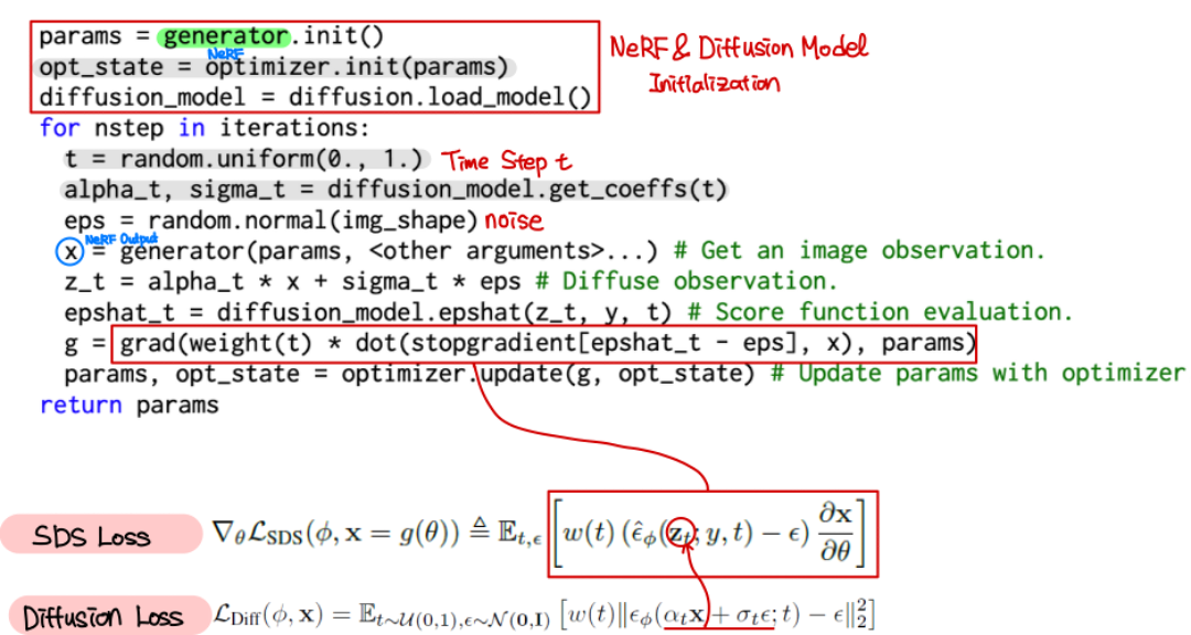
The entire process is an iterative optimization. We start with a NeRF whose weights θ are random noise, and we gradually refine them. The DreamFusion paper outlines a simple yet powerful four-step loop that we'll be implementing.

As you read, you'll see the core loop is elegantly straightforward: for a set number of iterations, we repeatedly:

1. Sample a Random Scene: Choose a random camera angle and lighting for the scene.
2. Render an Image: Use the current NeRF g(θ) to render a 2D view x based on the sampled camera.
3. Compute the SDS Loss: Calculate the loss (and its gradient) by comparing the rendered image x to the text prompt y using the SDS mechanism you learned previously.
4. Update the NeRF: Apply the gradient to the NeRF's parameters θ using an optimizer, nudging the 3D model to better match the prompt.

Let's break down each of these steps from an implementation perspective.

2. Anatomy of the Text-to-3D Training Loop

We will now detail the practical steps required to build this loop. We'll follow the algorithm's structure and incorporate key implementation details from both the original paper and the popular stable-dreamfusion open-source project.

Step 0: Initialization

Before the loop begins, we need to set up our environment:

• NeRF Model: Instantiate your 3D representation. In modern implementations like stable-dreamfusion, this is often a hash-grid-based NeRF (like the one from NVIDIA's Instant-NGP) for efficiency. The weights θ are initialized randomly.
• Optimizer: Initialize an optimizer for the NeRF parameters θ. While Adam is common, high-performance optimizers like Adan (used by stable-dreamfusion) or Distributed Shampoo (used in the original paper) are often chosen.
• Diffusion Prior: Load the pre-trained 2D text-to-image diffusion model. This is typically a model like Stable Diffusion, loaded from a library such as Hugging Face's diffusers. This model's weights are frozen; we only use it for inference.

Step 1: Random Camera and Light Sampling

At each iteration, we need to view our NeRF from a different angle. This is crucial for building a coherent 3D shape rather than a flat image that only looks good from one direction.

The DreamFusion paper specifies a robust sampling strategy:

• Camera Position: Sample a camera position in spherical coordinates.
  • Azimuth θ_cam: Uniformly sampled from [0°, 360°]. This covers all sides of the object.
  • Elevation φ_cam: Sampled from a range like [-10°, 90°]. This allows views from slightly below, at eye level, and from directly above.
  • Distance: Sampled from a range around the object's bounding sphere, ensuring we get both close-up and wider views.
• Light Position: Randomly sample a point light source, often positioned near the camera to create varied shading conditions.

This randomness ensures that the NeRF is optimized to look plausible from all angles and under different lighting, forcing it to learn a true 3D geometry.

Step 2: Differentiable Rendering

With a camera pose and light defined, you perform the step from our earlier lesson: render an image x = g(θ).
The stable-dreamfusion implementation renders at a low resolution (e.g., 64x64 or 128x128) during training to keep the process fast. The original paper also mentions a clever trick: sometimes rendering the full shaded color, and other times rendering just the textureless shape or the albedo. This helps disentangle geometry from appearance during learning.

Step 3: Diffusion Loss with View-Dependent Conditioning

This step contains the "magic" of SDS, but with a crucial twist for 3D. A text prompt like "a high-quality photo of a squirrel" usually implies a frontal view. If the camera is looking at the object from behind, the prompt is no longer accurate.

To solve this, we append view-dependent modifiers to the text prompt based on the sampled camera angle:

• If φ_cam is high (e.g., > 60°), append "overhead view".
• Based on the azimuth θ_cam, append "front view", "side view", or "back view".

The full prompt given to the diffusion model might become "a high-quality photo of a squirrel, back view". This gives the 2D diffusion model the correct context to judge the rendered image.

With the conditioned prompt, you then execute the SDS loss calculation as you learned in the last lesson:

1. Add noise ε to the rendered image x to get x_t.
2. Predict the noise ε_pred using the diffusion U-Net with Classifier-Free Guidance (CFG).
3. Calculate the gradient ∇_x L ∝ (ε_pred - ε).

Step 4: Optimization

The gradient is now automatically backpropagated through the rendering function g to the NeRF parameters θ (∂x/∂θ). A single optimizer step is taken:

# Pseudocode
loss = compute_sds_loss(rendered_image, prompt_with_view)
loss.backward()
optimizer.step()
optimizer.zero_grad()

This single step slightly improves the NeRF parameters θ so that the next time a similar view is rendered, it will be a little closer to what the diffusion model expects. After thousands of iterations (e.g., 15,000, taking 1-2 hours), these small updates accumulate to form a complete 3D object.

3. Running the Training Loop in Practice

Now, let's see how this theoretical loop translates into a concrete, runnable command. The stable-dreamfusion repository is an excellent open-source implementation of these ideas.

The video demonstrates how to combine all the components using a single Python script. Let's examine the command used to launch the training loop.

The key command looks like this:
python main.py --text "a high quality photo of a hamburger" --workspace trial_hamburger -O

Let's dissect this:

• python main.py: This is the main script that contains our full training loop.
• --text "...": This provides the text prompt y that will guide the optimization.
• --workspace "...": This specifies a directory to save the trained NeRF checkpoints and final renders.
• -O: This is a shorthand flag for optimization settings. In this repo, it enables the efficient Instant-NGP backbone for the NeRF and enables fp16 mixed-precision training to reduce memory usage and speed up computation.

When you execute this command, you are launching the entire iterative process we've described. The script will loop for thousands of steps, continuously sampling camera views, rendering, calculating SDS loss, and updating the NeRF, until it converges on a 3D representation of a hamburger.

Conclusion

Congratulations! You have now assembled the entire text-to-3D training pipeline. You've seen how to combine a differentiable 3D representation (NeRF) with a 2D diffusion model prior (Stable Diffusion) inside an optimization loop to generate a 3D asset from scratch.

Key Takeaways:

• The text-to-3D training process is an iterative optimization loop that refines a randomly initialized NeRF.
• Each iteration involves sampling a random camera view, rendering an image, calculating the SDS loss against a prompt, and updating the NeRF's weights.
• View-dependent prompt conditioning (e.g., adding "side view") is a critical technique to ensure 3D consistency.
• Practical implementations like stable-dreamfusion use highly efficient NeRF backbones (Instant-NGP) and optimizers to make this process feasible on consumer hardware.

Next Lesson Preview:

As you might have guessed from the mini-exercise, getting perfect results from this process is not always straightforward. Often, the generated 3D models suffer from strange artifacts. In the next lesson, we will dive into debugging, focusing specifically on two common failure modes: the Janus problem (where an object has multiple "fronts") and other geometric inconsistencies. You will learn why these happen and explore strategies to mitigate them.