Volume Rendering Equation Implementation

1. The Rendering Equation: From Points to Pixels

Imagine for each of the N points we sampled along a single ray, we've queried a neural network. This network, our NeRF model, has returned a color ${\mathbf{c}}_i$ and a density ${\sigma }_i$ for each point $i$. Our task is to collapse these N sets of $(c_i,{\sigma }_i)$ values into one final RGB color for the ray.

This is achieved through volume rendering. The core idea is to treat the density $\sigma$ as the probability that light "hits" something and stops at that point. The color $\mathbf{c}$ is the color that is emitted if the light stops there.

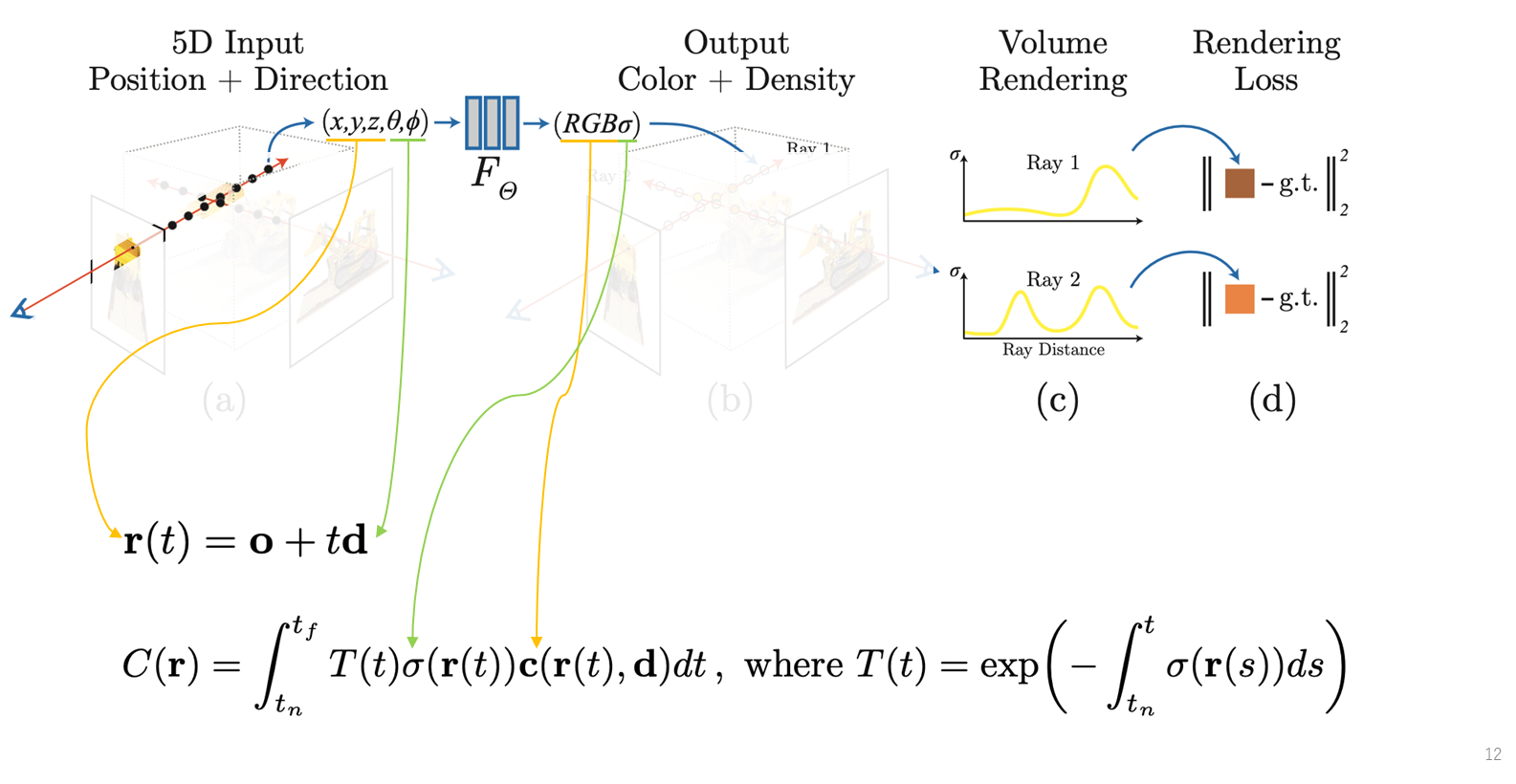
The discrete volume rendering equation synthesizes this intuition:

This equation might look complex, but it's built from a few simple, intuitive components that we'll implement one by one.

2. The Core Components of Volume Rendering

Let's break down the equation into its constituent parts. A fantastic article, "Key Parts and Codes(NeRF)", provides a clear explanation and a PyTorch implementation that we will follow.

After reviewing the material, let's solidify our understanding of the key terms:

• Distance (${\delta }_i$): This is the distance between adjacent sample points along the ray. We can compute this directly from the z_vals we generated in the previous lesson. ${\delta }_i=z_{i+1}-z_i$.

• Alpha (${\alpha }_i$): Also known as opacity. This value represents the probability that the ray terminates (i.e., is absorbed or reflected) within the segment $i$. It's a function of the density ${\sigma }_i$ and the segment length ${\delta }_i$.

  $${\alpha }_i=1-\exp (-{\sigma }_i{\delta }_i)$$

  A high density or a long segment length results in a high alpha, meaning the segment is more opaque.

• Transmittance ($T_i$): This is the probability that the ray travels from the camera all the way to segment i without being terminated by any of the preceding segments $1,2,...,i-1$. It is the cumulative product of the probabilities of passing through each prior segment.

  $$T_i=\prod _{j=1}^{i-1}(1-{\alpha }_j)$$

  If any preceding segment is highly opaque (high ${\alpha }_j$), the transmittance to subsequent segments drops significantly. For the first segment, $T_1=1$.

• Weights ($w_i$): This is the final contribution of sample $i$ to the pixel's color. It's the probability that the ray makes it to segment $i$ (transmittance) multiplied by the probability that it's stopped at segment $i$ (alpha).

  $$w_i=T_i\cdot {\alpha }_i$$

  The collection of weights $\{w_i\}$ for a ray forms a probability distribution, representing where along the ray the color is expected to originate.

The final pixel color, $\hat{C}(\mathbf{r})$, is simply the weighted sum of the colors of all samples along the ray: $\sum w_i{\mathbf{c}}_i$.

3. PyTorch Implementation

Now, let's translate this theory into a PyTorch function. The volume_rendering function from the Medium article you just read is an excellent template. Below is a breakdown of that implementation, connecting each line of code back to the concepts we just discussed.

Let's assume our inputs are:

• rgb: A tensor of shape [n_rays, n_samples, 3] containing the color for each sample.
• sigma: A tensor of shape [n_rays, n_samples] with the density for each sample.
• z_vals: A tensor of shape [n_rays, n_samples] with the depth of each sample.

import torch

def volume_rendering(
    rgb: torch.Tensor,
    sigma: torch.Tensor,
    z_vals: torch.Tensor
) -> torch.Tensor:
    """
    Computes the final color of a ray using the volume rendering equation.
    """
    # 1. Calculate distances (delta_i) between adjacent samples.
    dists = z_vals[..., 1:] - z_vals[..., :-1]
    # Append a large value for the last distance to simulate infinity.
    dists = torch.cat([dists, 1e10 * torch.ones_like(dists[..., :1])], dim=-1)

    # 2. Calculate alpha values (opacity).
    # ReLU on sigma ensures densities are non-negative.
    alpha = 1.0 - torch.exp(-torch.relu(sigma) * dists)
    
    # 3. Calculate transmittance (T_i).
    # torch.cumprod computes the cumulative product. We add a small epsilon
    # for numerical stability.
    transmittance = torch.cumprod(
        torch.cat([
            torch.ones((alpha.shape[0], 1), device=alpha.device),
            1.0 - alpha + 1e-10
        ], dim=-1),
        dim=-1
    )[:, :-1]
    
    # 4. Calculate weights (w_i).
    weights = alpha * transmittance
    
    # 5. Compute the final pixel color as the weighted sum of RGB values.
    rgb_map = torch.sum(weights.unsqueeze(-1) * rgb, dim=-2)
    
    return rgb_map

Implementation Notes:

• In step 1, appending 1e10 to dists is a practical trick to handle the last sample point. It simulates the idea that the ray travels to infinity beyond the last point, ensuring its contribution is properly accounted for.
• In step 3, we use torch.cat to prepend a 1 to the (1.0 - alpha) tensor. This establishes the base case $T_1=1$ before the cumulative product is computed. The 1e-10 epsilon prevents numerical instability if an alpha value is exactly 1.
• The use of unsqueeze in step 5 is a standard PyTorch operation to align tensor dimensions for broadcasting during the element-wise multiplication of weights (shape [n_rays, n_samples]) and rgb (shape [n_rays, n_samples, 3]).

To see this in the context of a complete rendering function, this short video is very effective.

4. Rendering More Than Just Color

The weights $\{w_i\}$ are incredibly useful. They represent a probability distribution along the ray. We can use this same distribution to compute a weighted average of any property of the sample points.

A common and useful example is rendering a depth map. Instead of compositing colors, we composite the depth values (z_vals) of each sample:

In code, this is a single line:
depth_map = torch.sum(weights * z_vals, dim=-1)

This gives us the expected depth of the surface for each pixel, which is invaluable for debugging the geometry your model has learned.

Conclusion

Congratulations! You have now implemented the final piece of the NeRF rendering puzzle. By combining the principles of stratified sampling and volume rendering, we can now transform a scene represented by a neural network into a 2D image.

Key Takeaways:

• The volume rendering equation is a differentiable method to composite color and density from sampled points into a final pixel color.
• The process relies on calculating alpha (opacity) and transmittance for each sample segment along a ray.
• The final weight for a sample, $w_i=T_i\cdot {\alpha }_i$, represents its total contribution to the pixel, naturally handling occlusion.
• This entire process can be implemented efficiently in PyTorch using vectorized operations like torch.cumprod.
• The same weights can be used to render other properties, such as a depth map, by taking a weighted average of the sample depths.

Next Lesson Preview:

We have now concluded our deep dive into the core components of Neural Radiance Fields. We understand how to represent a scene with an MLP and render it from any viewpoint.

In the next module, we will make a significant leap and connect this 3D knowledge back to your primary goal: diffusion models. We will begin exploring Text-to-3D Object Generation. Specifically, you will learn about Score Distillation Sampling (SDS), the groundbreaking technique used in models like DreamFusion. You'll see how a pre-trained 2D text-to-image diffusion model can be used to "teach" or "distill" its knowledge into a 3D representation like a NeRF, allowing you to generate 3D objects from nothing but a text prompt.