Stratified Sampling of Camera Rays

1. From Continuous Rays to Discrete Points

The core idea of volume rendering is to calculate the color of a pixel by integrating color and density contributions along the corresponding camera ray. The volume rendering equation, which we'll implement in the next lesson, is an integral:

As you know from your machine learning background, we often approximate integrals with a summation, similar to how expectation is approximated with a sample mean. This is exactly what we'll do here. We will approximate this integral using numerical quadrature, which involves evaluating the function at a discrete number of points and computing a weighted sum.

Our task today is to select these discrete points along the ray $\mathbf{r}(t)=\mathbf{o}+t\mathbf{d}$. The sampling process is bounded by two planes: a near plane ($t_{near}$) and a far plane ($t_{far}$). These define the volume of interest for our scene.

2. Stratified Sampling: A Smart Way to Sample

The simplest way to pick points would be to divide the segment from near to far into $N_c$ equal sections and pick the midpoint of each. This is uniform sampling. However, NeRF uses a slightly more clever technique called stratified sampling.

Stratified sampling works in two steps:

1. Partition: The interval $[t_{near},t_{far}]$ is divided into $N_c$ uniform, non-overlapping bins.
2. Sample: Instead of picking a fixed point in each bin (like the midpoint), we draw one sample uniformly at random from within each bin.

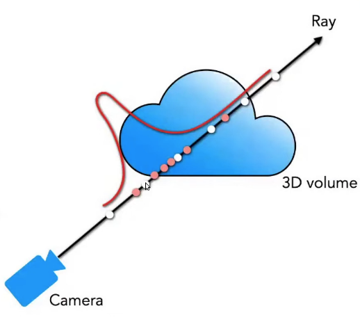
This image from 'The Annotated NeRF' article illustrates the difference between initial sampling and a refined sampling strategy. The white points represent the initial, evenly-spaced samples from stratified sampling, which we are implementing today. The red points show a later refinement step (hierarchical sampling), where more points are sampled in important regions.

Why bother with the randomness?
During training, the network sees slightly different 3D points for the same ray in every epoch. This prevents the model from overfitting to a fixed, discrete set of locations and forces it to learn a continuous representation of the scene's geometry and appearance. It acts as a form of regularization and reduces aliasing artifacts.

Let's hear a quick justification for this from a practical standpoint.

3. Implementing Stratified Sampling

Now, let's dive into the implementation. The "NeRF From Nothing" Google Colab notebook provides a clear and well-documented PyTorch function that does exactly what we need.

4. Code Walkthrough and Analysis

Let's dissect the sample_stratified function you just reviewed. It takes the ray origins and directions, near/far bounds, and the number of samples as input, and outputs the 3D points and their corresponding depth values.

Here is a slightly simplified version of the core logic:

import torch

def sample_stratified(rays_o: torch.Tensor,
                      rays_d: torch.Tensor,
                      near: float,
                      far: float,
                      n_samples: int,
                      perturb: bool = True):
    # 1. Create partition boundaries
    t_vals = torch.linspace(0., 1., n_samples, device=rays_o.device)
    z_vals = near * (1. - t_vals) + far * (t_vals)
    # z_vals are now the evenly spaced bin boundaries from near to far

    # 2. Get random samples within each bin
    if perturb:
        # Get midpoints between the bin boundaries
        mids = .5 * (z_vals[1:] + z_vals[:-1])
        
        # Define the lower and upper bounds of each bin
        upper = torch.concat([mids, z_vals[-1:]], -1)
        lower = torch.concat([z_vals[:1], mids], -1)
        
        # Draw a random sample 't' from Uniform(0, 1) for each bin
        t_rand = torch.rand([n_samples], device=z_vals.device)
        
        # Linearly interpolate between lower and upper bounds to get the final sample
        z_vals = lower + (upper - lower) * t_rand

    # Expand z_vals to match the batch dimension of rays
    z_vals = z_vals.expand(list(rays_o.shape[:-1]) + [n_samples])
    
    # 3. Compute 3D point locations: r(t) = o + t*d
    # rays_o: [batch_size, 3] -> [batch_size, 1, 3]
    # rays_d: [batch_size, 3] -> [batch_size, 1, 3]
    # z_vals: [batch_size, n_samples] -> [batch_size, n_samples, 1]
    pts = rays_o[..., None, :] + rays_d[..., None, :] * z_vals[..., :, None]
    # pts shape: [batch_size, n_samples, 3]
    
    return pts, z_vals

Key Implementation Points:

• Step 1 (Partitioning): torch.linspace creates values from 0 to 1, which are then linearly mapped to the [near, far] range. At this point, z_vals holds the edges of our bins.
• Step 2 (Perturbation): This if perturb: block is the "stratified" part. It defines the lower and upper boundary for each bin and then draws a random sample within it. This is a practical application of inverse transform sampling for a uniform distribution.
• Step 3 (Point Calculation): The final line pts = ... is the vector equation $\mathbf{r}(t)=\mathbf{o}+t\mathbf{d}$. The None indexing (... , None, :) is crucial for broadcasting the tensors to the correct shapes so that PyTorch performs the operation for every sample on every ray in the batch. The result is pts, a tensor of 3D coordinates.

The inverse_depth Parameter

You may have noticed an inverse_depth boolean in the Colab function. When set to True, it samples points that are linearly spaced in disparity (1/depth) rather than depth.

z_vals = 1. / (1./near * (1.-t_vals) + 1./far * (t_vals))

This is a useful trick. It allocates more samples to objects closer to the camera and fewer to objects far away, which can be a more efficient distribution of your fixed number of samples, especially for scenes with large depth variations. For now, we'll stick to linear depth sampling.

Conclusion

Excellent work! We have now built the second major component of our renderer. We started with rays and have now generated sets of 3D query points along each one.

Key Takeaways:

• Volume rendering approximates a continuous integral with a discrete sum, which requires sampling points along each camera ray.
• Stratified sampling is used to do this. It involves partitioning the ray segment [near, far] into bins and drawing one random sample from each bin.
• This randomness acts as regularization, preventing the model from overfitting to fixed points and helping to reduce aliasing.
• The implementation boils down to generating bin boundaries, perturbing them randomly, and then applying the ray equation $\mathbf{r}(t)=\mathbf{o}+t\mathbf{d}$ to get the final 3D point coordinates (pts) and their depth values (z_vals).

Next Lesson Preview:

We are now perfectly set up for the grand finale of the rendering module. We have our rays (rays_o, rays_d) and the points to evaluate (pts, z_vals). In the next lesson, we will implement the volume rendering equation. This involves taking the color and density predictions from our (hypothetical) NeRF model at each point pts and combining them using the principles of volumetric compositing to calculate the final, single color for the pixel.