Classifier Guidance and Classifier-Free Guidance

1. The Two Flavors of Guidance

At its core, "guidance" is about steering the generative process. Instead of letting the model generate a random image, we want to direct it to produce an image that adheres to a specific condition, like a class label or a text prompt.

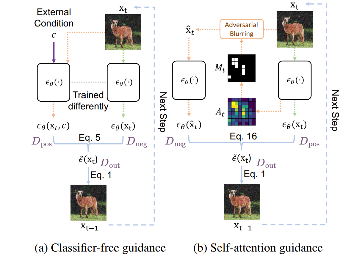
The diagram below illustrates the two main approaches we'll discuss. Pay attention to panel (a), Classifier-free guidance, as that will be our primary implementation goal.

2. Classifier Guidance: Steering with an External Expert

Before CFG became standard, the primary method for guidance involved using a second, separate model: a classifier.

The core idea is this:

• You have your main diffusion model, which is an expert at generating plausible images (denoising).
• You have a separate classifier model, which is an expert at identifying the class of an image. Importantly, this classifier must be trained on noisy images, so it can function at any step $t$ of the diffusion process.

At each sampling step, you use the gradient of the classifier to "nudge" the generation. The diffusion model makes a prediction for the denoised image, and then you adjust that prediction by moving it slightly in the direction that most increases the probability of the target class, according to the classifier.

This is mathematically derived from Bayes' theorem, where the reverse process $p(x_{t-1}|x_t,y)$ is guided by the classifier's belief $p(y|x_t)$.

Why isn't this the standard anymore?
While effective, classifier guidance has significant practical drawbacks:

• Training Overhead: It requires training and maintaining a separate, noise-aware classifier model.
• Architectural Complexity: The classifier must be compatible with the intermediate noisy images produced by the diffusion model.
• Adversarial Risk: The process can sometimes over-optimize for the classifier's belief, leading to images that fool the classifier but appear unnatural or distorted to a human eye.

This led researchers to ask: can we get the benefits of guidance without the classifier?

3. Classifier-Free Guidance (CFG): Guiding with the Model Itself

Classifier-Free Guidance is an elegant solution that eliminates the need for a second model. It leverages the dual-purpose model we built in the last lesson—one trained with conditioning dropout.

The key insight is that the difference between the model's conditional prediction and its unconditional prediction represents the direction of the guidance.

1. Unconditional Prediction (${ϵ}_{\theta }(x_t,\varnothing )$): This is the noise the model thinks should be removed to create any plausible image. It's the model's learned prior over the data distribution.
2. Conditional Prediction (${ϵ}_{\theta }(x_t,c)$): This is the noise the model thinks should be removed to create an image of a specific class or condition $c$.

The vector pointing from the unconditional to the conditional prediction, ${ϵ}_{\theta }(x_t,c)-{ϵ}_{\theta }(x_t,\varnothing )$, is essentially the "guidance signal" learned implicitly by the model.

CFG combines these predictions to create a new, guided estimate of the noise, ${\widetilde{ϵ}}_{\theta }$:

Here, $s$ is the guidance scale (also often denoted as $w$).

• If $s=0$, we get purely unconditional generation: ${\widetilde{ϵ}}_{\theta }={ϵ}_{\theta }(x_t,\varnothing )$.
• If $s=1$, we get the standard conditional generation: ${\widetilde{ϵ}}_{\theta }={ϵ}_{\theta }(x_t,c)$.
• If $s>1$, we extrapolate along the guidance direction, amplifying the condition. This pushes the generation to be more like the target class than what the model might have produced with $s=1$.

4. Implementing CFG in the Sampling Loop

Now for the practical part. Implementing CFG involves modifying your sampler (e.g., DDIM, DPM-Solver) to compute and use the guided noise estimate ${\widetilde{ϵ}}_{\theta }$ at each step.

The following resource provides a step-by-step guide to this modification.

To summarize the key implementation steps within your sampling loop for a single batch:

1. Duplicate Inputs: For a batch of size B, you need to prepare inputs for a single, larger forward pass.

   • The noisy image tensor x_t (shape [B, C, H, W]) is duplicated to create a tensor of shape [2*B, C, H, W].
   • The timestep tensor t is similarly duplicated.
   • The condition tensor c and the null condition tensor null_c are concatenated to form a conditioning tensor of shape [2*B, ...].

2. Single Forward Pass: Pass these concatenated tensors through your U-Net in one go.
   noise_pred_combined = model(torch.cat([x_t] * 2), ..., torch.cat([c, null_c]))

3. Split Predictions: Split the output from the model back into two parts.
   noise_pred_uncond, noise_pred_cond = noise_pred_combined.chunk(2)

4. Apply CFG Formula: Use the guidance scale to compute the final noise prediction.
   predicted_noise = noise_pred_uncond + guidance_scale * (noise_pred_cond - noise_pred_uncond)

5. Proceed with Sampler: Use this predicted_noise in the rest of your sampler's logic (e.g., to predict ${\hat{x}}_0$ and compute $x_{t-1}$ in a DDIM step).

This approach roughly doubles the inference cost per step, as you're effectively doing two forward passes, but the improvement in control and quality is almost always worth it.

For an alternative implementation view within a full class structure, you can refer to the get_img_latents method in the article "How to Generate Images from Text using Stable Diffusion" (LINK), which you can find in the provided resources.

import torch

def sampling_step(model, x_t, t, condition, null_condition, guidance_scale):
    """
    Performs one step of denoising.
    x_t: The current noisy image tensor, shape [B, C, H, W]
    t: The current timestep
    condition: The conditional embedding, shape [B, embed_dim]
    null_condition: The unconditional (null) embedding, shape [B, embed_dim]
    guidance_scale: The guidance scale 's'
    """
    
    # --- Current implementation (conditional only) ---
    # predicted_noise = model(x_t, t, condition) 
    
    # --- YOUR MODIFICATION HERE ---
    # Implement CFG to calculate 'predicted_noise'
    # You should use x_t, t, condition, null_condition, and guidance_scale

    predicted_noise = None # Replace this

    # --- END OF MODIFICATION ---

    # (The rest of the sampler logic would use predicted_noise)
    return predicted_noise

    # --- YOUR MODIFICATION HERE ---
    # 1. Prepare batched inputs for the model
    latent_model_input = torch.cat([x_t] * 2)
    time_input = torch.cat([t] * 2) # Assuming t is a tensor of shape [B]
    condition_input = torch.cat([null_condition, condition])

    # 2. Perform a single forward pass
    with torch.no_grad():
        noise_pred_combined = model(latent_model_input, time_input, condition_input)
    
    # 3. Split the predictions
    noise_pred_uncond, noise_pred_cond = noise_pred_combined.chunk(2)
    
    # 4. Apply the CFG formula
    predicted_noise = noise_pred_uncond + guidance_scale * (noise_pred_cond - noise_pred_uncond)

5. The Impact of the Guidance Scale

The guidance scale $s$ is a powerful hyperparameter that you will frequently tune. It controls the trade-off between how strictly the model adheres to the condition and the overall diversity/quality of the output.

• Low Scale (e.g., 1-4): Produces diverse and often high-quality images, but they might not follow the condition (e.g., class label or text prompt) very closely.
• Medium Scale (e.g., 5-10): This is often the sweet spot, providing a good balance between condition adherence and image quality. Most text-to-image models default to a value in this range (e.g., 7.5).
• High Scale (e.g., 11-20+): Forces the model to adhere very strictly to the condition. This can be useful, but often leads to image saturation, strange artifacts, and a sharp drop in diversity, as the model is pushed far beyond the distributions it saw during training.

Conclusion

You have now explored the theory behind guidance and the practical implementation of Classifier-Free Guidance, a cornerstone of modern conditional diffusion models.

Key Takeaways:

• Classifier Guidance uses an external, noise-aware classifier's gradients to steer generation but is complex and less common now.
• Classifier-Free Guidance (CFG) achieves superior results without a second model by leveraging a diffusion model trained with conditioning dropout.
• The CFG formula, ${\widetilde{ϵ}}_{\theta }={ϵ}_{\theta }(x_t,\varnothing )+s\cdot ({ϵ}_{\theta }(x_t,c)-{ϵ}_{\theta }(x_t,\varnothing ))$, extrapolates from the unconditional prediction in the direction of the conditional one.
• The implementation is efficient, requiring a single forward pass on a doubled batch at each inference step.
• The guidance scale ($s$) is a critical hyperparameter for balancing fidelity to the condition against sample quality and diversity.

Next Lesson Preview:

Knowing how to implement CFG is the first step. The next is mastering its use. In our next lesson, we will focus on how to tune the CFG scale and diagnose common artifacts arising from guidance. You will learn to identify the visual signatures of a guidance scale that is too high or too low, enabling you to debug and refine your generations for optimal quality.